Engineering Mathematics · Calculus for ML
Loss Landscapes
In Engineering Mathematics because training a model is literally moving through a loss surface whose slopes, flats, and valleys decide optimization behavior.
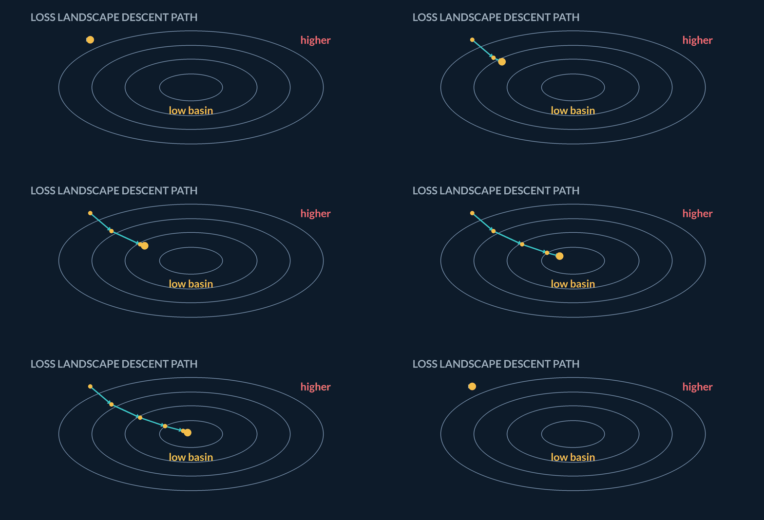
This topic specializes the surface idea to machine learning. The height is loss, the coordinates are model parameters, and training is the process of moving to lower parts of that landscape.
- Engineering Mathematics
- Medium level
- 4 concepts
1Training moves in parameter space, not data space
A loss landscape is the graph of model error as a function of the parameter vector. Each point in that space is one full model setting, and the height says how bad that setting is on the chosen objective.
This picture explains why training can speed up, stall, or zig-zag. Those behaviors reflect geometry of the loss surface: flat regions, narrow valleys, curved walls, and saddle structures in parameter space.
Figure. A one-parameter loss landscape is a bowl over parameter values. Training moves along the parameter axis seeking lower loss.
Read the axes
- Choose parametersEach coordinate is a model parameter or a parameter vector.
- Evaluate lossThe height at that coordinate is the objective value on the chosen data.
- Move by updatesTraining changes coordinates, not the training examples themselves.
One point in parameter space
A one-parameter model uses \hat y=wx. For data (1,2) and (2,4), compute the MSE height at w=1.5.
- Predictions at w=1.51.5 and 3.0
- Errors1.5-2=-0.5 and 3.0-4=-1.0
- Squared errors0.25 and 1.00
- MSE(0.25+1.00)/2=0.625
Pro tip. The point w=1.5 is one model setting; its landscape height is 0.625 on this dataset.
Model yhat=wx on data (1,2),(2,4). What is MSE at w=1?
- 2.5
- 0
- 1.5
- 5
Predictions are 1,2, residuals are -1,-2, squared errors 1,4, average 2.5.
2Candidate weights are compared by their losses
A loss landscape becomes concrete when you compute the loss for two candidate parameter values on the same examples. The lower point is the better fit for that objective.
This is the simplest version of model selection during training: not by how the line looks in isolation, but by the objective value it produces on the data.
Figure. Candidate weights are compared by the same loss on the same data. The zero-height bar marks the exact fit in this tiny example.
Compare two weights
- Fix dataUse the same examples for both candidate weights.
- Compute predictionsApply \hat y=wx for each candidate.
- Average squared errorsCompute MSE and pick the lower value.
MSE for two candidate weights
Use data (x,y)=(1,2),(2,4),(3,6) and model \hat y=wx. Compare w=1 and w=2.
- For w=1, predictions1,2,3
- For w=1, squared errors(1-2)^2,(2-4)^2,(3-6)^2 = 1,4,9
- MSE at w=1(1+4+9)/3=14/3\approx4.67
- For w=2, predictions2,4,6
- MSE at w=20, so w=2 is lower
Pro tip. The lower landscape point is w=2 for this data and this objective.
For the same data (1,2),(2,4), compare w=1 and w=2.
- w=2 has lower MSE
- w=1 has lower MSE
- They tie
- MSE cannot compare weights
w=2 predicts 2,4 exactly, while w=1 has nonzero residuals.
3Repeated loss values reveal the valley
A loss landscape is not known from one point. Computing loss at several parameter values reveals whether the objective is falling, rising, or forming a valley.
For a simple linear model on perfectly linear data, the MSE values shrink as the weight approaches the matching slope and grow as the weight moves away.
Sample the landscape
- Choose candidatesPick several parameter values on the same axis.
- Compute each lossUse the same data and objective every time.
- Read patternLook for the lower region and how sharply loss rises away from it.
Three sampled heights on the same loss curve
For data (1,2),(2,4),(3,6) and \hat y=wx, compare w=1.5, w=2, and w=2.5.
- At w=1.5, errors-0.5,-1.0,-1.5
- MSE at w=1.5(0.25+1+2.25)/3=3.5/3\approx1.17
- MSE at w=20
- At w=2.5, errors0.5,1.0,1.5
- MSE at w=2.5(0.25+1+2.25)/3\approx1.17
Pro tip. The equal losses at 1.5 and 2.5 show a symmetric one-parameter valley around w=2 for this dataset.
Coding lab. Plot a one-parameter loss valley runs in the app, with checks on your output.
Losses at w=0,1,2 are 9,1,9. What does this suggest?
- A valley centered near w=1
- A flat region everywhere
- A maximum at w=1
- No parameter landscape
The middle sampled point is much lower and both sides rise, indicating a valley around w=1.
4Flat and steep regions change optimization behavior
The same update size behaves differently in different parts of a loss landscape. In a flat region, nearby losses change slowly; in a steep region, the same parameter move can change loss sharply.
This matters because optimizers use local slope information. A small slope can make progress slow, while a very steep slope can make an aggressive step overshoot.
Figure. The same horizontal parameter move can barely change loss in a flat region and sharply change it in a steep region. This is the visual meaning of gradient magnitude.
Compare local changes
- Pick nearby weightsCompare small moves near a low point and farther away.
- Compute loss changesUse the same MSE objective.
- Interpret slopeSmall changes imply a flatter region; large changes imply a steeper region.
Flat near the valley, steep farther away
Using the same data (1,2),(2,4),(3,6) and \hat y=wx, compare MSE changes from w=2 to 2.1 and from w=3 to 3.1.
- MSE at w=2.1(0.01+0.04+0.09)/3\approx0.047
- Change from w=2 to 2.10.047-0=0.047
- MSE at w=3(1+4+9)/3\approx4.67
- MSE at w=3.1(1.21+4.84+10.89)/3\approx5.65
- Change from w=3 to 3.15.65-4.67=0.98
Pro tip. The same 0.1 weight move changes loss much more far from the valley than near the bottom.
A 0.1 step changes loss by 0.01 near one point and by 1.2 near another. Which region is steeper?
- The second region
- The first region
- They are equally steep
- Neither has a gradient
The same parameter move causing a larger loss change indicates a steeper local region.
Notes
- A loss landscape maps parameter settings to an error value that training tries to reduce.
- Flat regions, steep directions, valleys, and saddles all affect how optimization feels in practice.
- Candidate parameter values can be compared by computing the loss on the same data points.
Formulas
- L(theta) assigns one loss value to each parameter vector theta.
- For predictions yhat_i, MSE = (1/n) sum_i (yhat_i - y_i)^2.
- For a one-parameter linear model yhat = wx, the landscape is the curve L(w).
Exam traps & shortcuts
- The landscape metaphor is only useful if you remember the axes are parameters, not input examples.
- Always compare candidate losses on the same data; changing the data changes the landscape.
Reference tables
Use the same objective and data whenever comparing points on a loss landscape.
| Step | Question |
|---|---|
| Axes | Which parameters define this point? |
| Height | What loss is computed at that parameter setting? |
| Comparison | Which candidate has lower loss on the same data? |
| Geometry | Do nearby losses change slowly, sharply, or asymmetrically? |
Recap
Loss landscapes make optimization language concrete.
- Axes
- A loss landscape is drawn over parameter space, with height equal to model error.
- Behavior
- Optimization behavior mirrors the local geometry of that landscape.
- Compare
- Candidate weights are compared by computing the same loss on the same data.
- Valley
- Sampling several parameter values reveals low regions and how steeply loss rises away from them.
Practise Loss Landscapes
Reading is free and needs no account. Practice, mocks and progress live in the app.
- A 5-question practice set that ends the chapter
- 4 quick checks with worked explanations
- Timed mocks scored with the real marking scheme
- Readiness tracked per topic, kept on your device