Artificial Intelligence · AI Foundations
Cost-Aware Search
In AI because cost-aware search — uniform-cost, which is Dijkstra on an implicit graph — computes provably optimal plans whenever the model is known, no learning needed.
Real routes are not measured in hops: edges carry costs — minutes, joules, rupees, risk — and the plan that matters is the one whose total is smallest. This lesson builds uniform-cost search, which is Dijkstra's algorithm let loose on graphs too large to write down, and shows exactly why cheapest-total-first is allowed to stop the moment the goal is popped.
- Artificial Intelligence
- Medium level
- 7 concepts
1Path cost is the objective
A search problem so far scored a plan by its length — the number of edges. Real problems price each edge: a weight is minutes of driving, joules of battery, rupees of toll, or any other quantity that adds along a route. The path cost g(n) is that running sum from the start to n, and the object of cost-aware search is the plan whose total is smallest, not the plan with the fewest moves.
The two objectives disagree the moment weights are unequal. On the lesson graph the direct edge from S to G is the shortest plan by hops — one move — and not the cheapest by cost; the two-edge route through B doubles the moves and still undercuts it at 8 against 10. Hop count is just path cost with every edge priced 1, which is why breadth-first search is the special case and uniform-cost search the general one.
Figure. Three complete routes to the same goal. The route via A opens with the cheapest edge on the graph (2) and still totals dearest at 11; the winner is the route whose completed total is smallest — 8 via B. Only completed totals compare.
Fewest hops picks the direct edge; least cost picks the route through B.
| Route | Hops | Total cost |
|---|---|---|
| S→G direct | 1 | 10 |
| S→A→G | 2 | 2 + 9 = 11 |
| S→B→G | 2 | 5 + 3 = 8 |
2Uniform-cost search
Uniform-cost search keeps a frontier of partial paths and always expands the one with the smallest path cost g so far. Cheapest-first is not an optimisation of the algorithm; it is the algorithm: pop anything else and the first path found to a node stops being its cheapest.
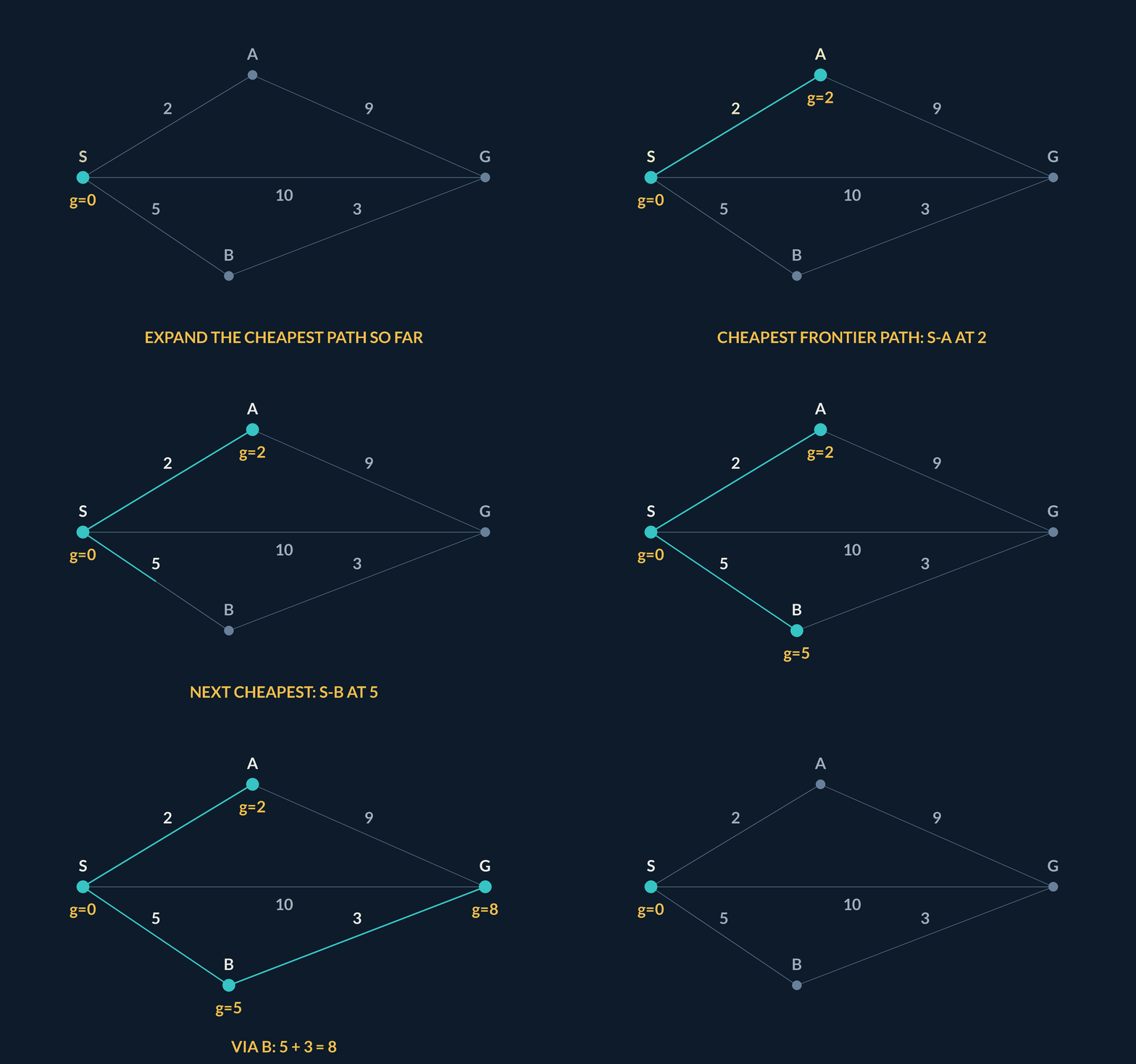
Two details carry the correctness. The frontier is a priority queue ordered by g, so a cheap first edge cannot commit the search to a dear route — the route through A opens promisingly at 2 and is quietly overtaken once its total passes 8. And the goal test happens when a node is popped, not when it is first generated: G is generated at cost 10 through the direct edge, but stopping there would lock in the wrong answer while the total of 8 was still in the queue.
Under one assumption — no edge cost is negative — the first time any node pops, its recorded g is the cheapest possible, so the search may settle it permanently and stop the moment the goal pops. That assumption gets its own scrutiny in the negative-costs lesson.
Three routes, one pop order
On the lesson graph (S→A 2, A→G 9, S→B 5, B→G 3, S→G 10), find the cheapest cost from S to G.
- S→A→G = 2 + 911
- S→B→G = 5 + 38
- direct S→G10
- pop order: S at 0, A at 2, B at 5, G at 8UCS returns 8
Pro tip. Watch what the search never did: it never compared routes. Ordering the frontier by g makes the comparison fall out of the pop order — G simply cannot pop at 10 while a total of 8 is queued.
Coding lab. Uniform-cost search on the lesson graph runs in the app, with checks on your output.
Uniform-cost search pops a node whose path cost is 12 while a node of cost 9 is still waiting on the frontier. What has gone wrong?
- Nothing: uniform-cost search pops in insertion order, not by cost
- The heuristic guiding the search must be inadmissible
- The graph must contain an edge with a negative cost
- The frontier is not ordered by cumulative cost, which is the single property the optimality of the search rests on
Cheapest-first is not an optimisation of this algorithm, it is the algorithm. Pop anything else and the first path found to a node stops being its cheapest.
3Dijkstra on an implicit graph
Uniform-cost search is Dijkstra's algorithm — the same priority queue, the same settle-on-pop — with one change of setting. Dijkstra as taught in an algorithms course walks a graph handed to it as an adjacency list. An AI planner cannot be handed the graph: the states of a puzzle, a logistics problem or a configuration space number beyond storage, so the graph exists only as a successor function that, shown a state, returns its neighbours and their costs on demand.
That changes what governs the running time. On an explicit graph the cost is about (V + E) \log V with a binary heap. On an implicit graph the search only ever materialises the ball of states cheaper than the optimum C^*, and with branching factor b and minimum edge cost \varepsilon that ball holds on the order of b^{1 + \lfloor C^*/\varepsilon \rfloor} nodes. The exponent is a budget: it counts how many cheapest edges fit under the optimum, so fine-grained costs — a small \varepsilon — inflate the space even when the graph and the answer are unchanged.
Figure. The same planner and the same optimal cost: halving the minimum edge cost from 1 to 0.5 deepens the cost ball from 10⁵ to 10⁹ nodes. The bars are on a log scale — each rung of the ladder is a factor of ten.
The cost ball
A planner branches b = 10 ways per state and the optimal plan costs C* = 4. Estimate the states touched when the minimum edge cost is ε = 1, and again when costs are graded at ε = 0.5.
- ε = 1: b^(1+⌊4/1⌋) = 10⁵100,000 nodes
- ε = 0.5: b^(1+⌊4/0.5⌋) = 10⁹1,000,000,000 nodes
- 10⁹ / 10⁵ — same graph, same optimum10,000× the work
Pro tip. ε is the step size of the cost lattice, not a property of the answer. When you design a cost model, coarsen it as far as honesty allows — every extra decimal place of cost resolution is potentially another factor of b.
4Why settled-when-popped is safe
Uniform-cost search makes a strong claim: the first time a node pops, its g is final — no reopening, no second thoughts. The proof is a cut argument, and it is worth holding in full because every variant question you will meet later (negative edges here, inconsistent heuristics in A*) is answered by asking which line of it broke.
Suppose node n pops with cost g(n), and some cheaper path to n exists. That path starts inside the settled set and ends outside it, so somewhere it crosses the boundary at a frontier node f. The queue popped n rather than f, so g(f) \ge g(n). The rest of the rival path runs from f to n through edges that are each non-negative, so it can only add: the rival totals at least g(f), which is at least g(n). The rival is no cheaper — contradiction, and the pop is safe.
Read the chain once more, slowly: it uses non-negative edges exactly once. That single use is the hinge the negative-costs lesson swings on.
Figure. n has just popped. Any rival route to n must leave the settled set through some frontier node f; the queue preferred n, so g(f) ≥ g(n), and the dashed remainder only adds. No rival can be cheaper — settling n is safe.
The cut argument
- Cross the boundaryAny rival path to n starts in the settled set and must exit it through some frontier node f.
- Pop order bounds fn popped first, and the queue is ordered by g, so g(f) ≥ g(n).
- Edges only addFrom f onward every edge is ≥ 0, so the rival totals ≥ g(f) ≥ g(n): never cheaper.
5Cost models: what the weights mean
The algorithm never asks what a cost is; the engineer must. A weight is a claim that the quantity adds along a route and that smaller is better — time, energy, money and risk all qualify once they share a unit. Mixing units without conversion, or folding two objectives into one number without deciding the exchange rate, produces plans that are optimal for a question nobody asked.
One conversion is used everywhere in production systems: probabilities multiply along a route, and −log turns multiplication into addition. Price each edge at −log p and the cheapest path is the most probable one — this is how speech decoders, spell correctors and translation lattices run Viterbi-style decoding as plain shortest-path search.
Keep the cost model separate from the heuristic in your head: the cost is the terrain, part of the problem's definition; a heuristic — the informed-search lesson's subject — is advice about the terrain, and only the advice is allowed to be wrong.
| Objective | An edge costs | Watch for |
|---|---|---|
| Time | minutes for that leg | waiting time belongs on the edge that waits |
| Energy | joules drawn | regenerative braking makes a negative edge — the negative-costs lesson covers it |
| Money | toll plus fuel for the leg | currencies must be converted, not mixed |
| Probability | −log p of the step | zero-probability edges price as infinite; prune them instead |
Most probable path as cheapest path
Two edges on a decoding lattice carry probabilities 0.9 and 0.5. Show that summing −ln p reproduces the route's probability.
- −ln 0.90.105
- −ln 0.50.693
- route cost = 0.105 + 0.6930.799
- −ln(0.9 × 0.5) = −ln 0.450.799 — the same number
Pro tip. The identity is exact, so the ranking is exact: cheapest −log total and most probable route are the same route, always. Note the byproduct — probabilities strictly between 0 and 1 give strictly positive costs, so the non-negativity assumption comes free.
6The frontier in practice
Between the textbook and a working planner sits one data-structure decision. The classic presentation of Dijkstra assumes a priority queue with decrease-key: when a cheaper path to a queued state appears, reach in and lower its key. Binary heaps — including Python's heapq — do not support that operation, and the production idiom is not to want it: push a duplicate entry with the better cost and let the stale one surface later.
The guard that makes duplicates safe is one comparison at pop time: if the popped g is worse than the best g recorded for that state, the entry is stale — skip it. Every skipped pop costs one heap operation; in exchange the code needs no handles into the middle of the heap, and the whole queue stays a few lines of standard library.
The other half of the frontier is the explored set, keyed by the state itself — which quietly assumes states are hashable and canonical. That assumption is load-bearing enough to get its own lesson: two encodings of the same situation that hash differently will both be expanded, and the search does every piece of work as many times as you failed to canonicalise.
Figure. A cheaper path to a queued state is pushed as a new heap entry; nothing reaches in to decrease-key. At pop, if that g exceeds the best recorded g for the state, the entry is stale — skip it. Stale pops change no answer.
Lazy deletion
- Push duplicatesA cheaper path to a queued state is pushed as a new entry; nothing reaches into the heap.
- Guard at popIf the popped g exceeds the best recorded g for that state, the entry is stale.
- Skip and continueStale pops cost one heap operation each and change no answer.
UCS with lazy deletion (heapq)
import heapq

def ucs(start, goal, successors):
    frontier = [(0, start)]          # (g, state); duplicates allowed
    best = {start: 0}                # cheapest g seen per state
    while frontier:
        g, s = heapq.heappop(frontier)
        if g > best.get(s, float('inf')):
            continue                 # stale entry - lazy deletion
        if s == goal:
            return g
        for nxt, w in successors(s):
            g2 = g + w
            if g2 < best.get(nxt, float('inf')):
                best[nxt] = g2
heapq.heappush(frontier, (g2, nxt))7When search beats learning
Cost-aware search assumes you hold the problem exactly: the states, the successor function and every edge cost are known and trusted. Where that holds — puzzles, routing on a mapped warehouse, dependency resolution, configuration — search computes the optimum directly, with a proof, and a learned policy could only approximate the same answer while adding data needs, training cost and failure modes.
Learning earns its cost precisely where the givens fail: the transition model is unknown (what does this action actually do?), the costs must be estimated (how long does this road take at 6 pm?), or the state is only partially observed. There, estimation is not overhead — it is the task.
The frontier of the field is mostly the hybrid strip between the two: a learned model predicts costs or ranks successors, and classical search runs on top of the predictions — traffic-trained travel times feeding an exact shortest-path engine, or game-tree search guided by a learned evaluation, which is the AlphaGo shape. The search half keeps the guarantees; the learned half keeps the model honest about the world.
| Problem | Model known and exact? | First reach |
|---|---|---|
| 8-puzzle, Sudoku, solvers | yes — the rules are the game | search |
| Routing on a surveyed map | yes — edges measured once | search |
| Routing under live traffic | costs drift with the hour | learned costs + search |
| Robot arm from camera pixels | transition model unknown | learning |
You hold a complete, exact map of a warehouse and need shortest routes for a robot. Why is a learned policy the wrong first reach?
- Reinforcement learning is too slow to run onboard a robot
- Search always executes faster at run time than a neural network
- A learned policy is incapable of representing a shortest path
- The moves and their costs are already known exactly, so search computes the optimum a policy could only approximate
Learning is how you cope with a transition model or cost you do not have. When you do have them, estimating them from experience throws away information you were given for free.
Notes
- Uniform-cost search expands the cheapest cumulative path first and is Dijkstra's algorithm run on an implicit graph.
- Optimality rests on one assumption: extending a path never lowers its cost.
- Search beats learning when the transition model and every cost are known exactly; hybrids put learned costs under a classical search.
Exam traps & shortcuts
- Order the frontier by cumulative g, never by insertion order or hop count.
- Test the goal when its node is popped, not when it is generated — a goal seen early may still have a cheaper path coming.
- A cheap first edge proves nothing about the route it starts; only completed totals compare.
Recap
This lesson in brief:
- Path cost is the objective
- Edges carry costs that add along a route; hop count is the special case where every edge costs 1.
- Uniform-cost search
- Expand the cheapest cumulative g first and test the goal at pop — on the lesson graph, 8 via B beats the direct 10 and the cheap-looking 11 via A.
- Dijkstra on an implicit graph
- Same algorithm, but the graph exists only as a successor function, and the work is the cost ball b^(1+⌊C*/ε⌋), not V and E.
- Settled when popped
- Any rival path crosses the frontier at some f with g(f) ≥ g(n) and then only adds — an argument that spends non-negativity exactly once.
- When search beats learning
- A known, exact model makes search the first reach; learning enters when the model or its costs must be estimated.
Practise Cost-Aware Search
Reading is free and needs no account. Practice, mocks and progress live in the app.
- 2 quick checks with worked explanations
- Timed mocks scored with the real marking scheme
- Readiness tracked per topic, kept on your device