Artificial Intelligence · AI Foundations
Search Problems and Breadth-First Search
In AI because posing a task as states, moves and a goal test — then exploring systematically — is classical intelligent behaviour that needs a model of the moves, not data or…
A search problem hands the computer three things — a starting state, the legal moves out of each state, and a test that recognises the goal — and asks for a path. Nothing is learned and no data is fitted: the intelligence is in exploring the space of states systematically instead of blundering through it. This lesson builds that framing, the bookkeeping every search shares, and breadth-first search — the strategy that buys a shortest-path guarantee and pays for it in memory.
- Artificial Intelligence
- Medium level
- 6 concepts
1What a search problem is
A search problem is a task rewritten in three parts: a state (a complete description of one situation), the actions that are legal in each state, and a goal test that recognises success. A solution is a path — the sequence of actions leading from the start state to a goal state — and when actions carry costs, an optimal solution is a cheapest such path.
The rewriting is where the intelligence lives. The 8-puzzle becomes searchable the moment a state is 'the arrangement of tiles' and an action is 'slide one tile into the blank'; a delivery run becomes searchable as 'the junction the van is at' and 'drive one road'. Together the states and actions form the state space — a graph the algorithm walks without ever seeing all of it at once.
Note what is absent: no examples, no labels, no training. Search needs a model of the moves, not data about past episodes, which is why planners, puzzle solvers and the lookahead inside game engines stay classical even in systems that use learning everywhere else.
Figure. The states reachable from the start and the legal moves between them form a graph — here with two routes to the goal, an upper one of three moves and a lower one of four. A search algorithm walks this graph from the start node; it never sees the whole map, only the neighbours of states it has already generated.
| Component | 8-puzzle | Delivery route |
|---|---|---|
| State | One arrangement of the eight tiles and the blank | The junction the van is at |
| Action | Slide a neighbouring tile into the blank | Drive one road segment |
| Goal test | Tiles read 1–8 in order | Van is at the customer's address |
| Path cost | Number of slides | Metres driven or minutes taken |
2The frontier and the explored set
Every search algorithm in this course — BFS here, depth-first in the next lesson, the cost-aware searches after that — is the same loop over two lists. Only the choice of which node to take next differs.
The frontier is the to-do list: states that have been generated (seen as somebody's neighbour) but not yet expanded (had their own neighbours generated). Take the oldest frontier node first and the loop is breadth-first; take the newest and it is depth-first — the data structure, a queue or a stack, is the entire personality of the algorithm.
The explored set is the done list: states already expanded, kept so that no state is expanded twice. It is what separates graph search from tree search, and it trades memory for termination — wherever two routes can reach the same state, tree search re-does the shared work exponentially often, and on a map with cycles it never stops at all.
The distinction between generated and expanded sounds pedantic and is not: the complexity counts, the goal-test placement and the correctness argument for BFS all hang on it.
Figure. A search frozen mid-run. The explored set (S, A, B) is finished and must not be revisited; the frontier (C, D, E) waits in the queue; dashed edges lead to states nobody has generated yet. Drop the explored set and you loop forever; drop the frontier and you forget where to go next.
| Structure | What it holds | What breaks without it |
|---|---|---|
| Frontier (to-do) | States generated but not yet expanded | Nothing records where to continue — there is no search left to run |
| Explored set (done) | States already expanded | Cycles recirculate states forever; shared states are re-expanded exponentially often |
You run a graph search with a frontier but no explored set, on a map containing cycles. What happens?
- The same states are pushed over and over, so the frontier keeps growing while the search makes no progress
- It still terminates, because the frontier eventually empties
- It terminates quickly but returns the wrong path
- Nothing changes, because the explored set is only a speed-up on trees
The frontier is a to-do list and nothing in it says a state has already been done. On a cyclic graph that omission turns a finite search into an unbounded one.
3Breadth-first search
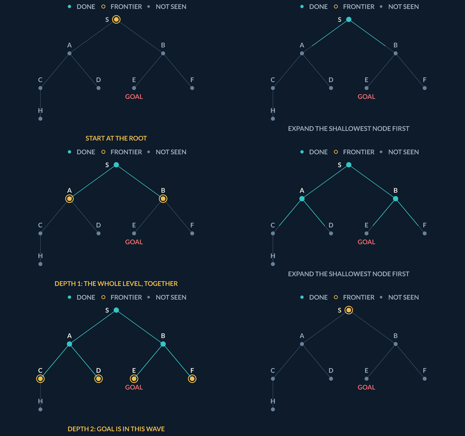
Breadth-first search expands the frontier oldest-first — a FIFO queue — which makes the search spread from the start in waves: every state one move away, then every state two moves away, never touching depth d+1 while a depth-d state still waits.
That discipline buys the guarantee the animation shows: the first time BFS reaches the goal, no shorter path exists, because every strictly shallower state has already been tried. The guarantee is about the number of moves — fewest moves equals cheapest route only when every move costs the same.
One implementation detail matters more than it looks: apply the goal test when a state is generated, not when it is dequeued for expansion. Testing at expansion leaves the goal sitting in the queue behind an entire level of siblings — at branching factor 10, up to ten times the work for nothing.
BFS is complete whenever the branching factor is finite: even on an infinite state space, a goal at depth d is reached after finitely many expansions, because only finitely many states are shallower.
Coding lab. Implement BFS and check it against networkx runs in the app, with checks on your output.
BFS returns the path with the fewest hops. On a road map whose edges carry travel times, what has it found?
- The fastest route, since crossing fewer roads means less travelling
- Nothing usable, because BFS cannot be run on a weighted graph at all
- A route crossing the fewest road segments, which can take far longer than a winding alternative
- The cheapest route, as long as every travel time is positive
BFS optimises hop count. That equals cost only when every edge costs the same, and a motorway hop and a village lane hop plainly do not.
4Why BFS is complete, and when it is optimal
Complete means: if any solution exists, the algorithm finds one. Optimal means: the first solution returned is a cheapest one. Neither is decoration — an engineer choosing a search needs to know which promises hold and under what conditions, because both are conditional.
Completeness: with a finite branching factor b, there are at most 1 + b + b^2 + \dots + b^d states within d moves of the start — finitely many. BFS expands shallowest-first, so if the nearest goal sits at depth d, it is reached after finitely many expansions even when the state space as a whole is infinite.
Optimality, unit costs: BFS expands states in non-decreasing depth — the queue never lets a deeper state overtake a shallower one. So when a goal is first generated, every state of smaller depth has already been generated and none of them passed the goal test; no shorter path was missed.
Both promises are conditional. Infinite branching breaks completeness, because some level can never be finished. Unequal action costs break optimality: the fewest-move path can be the dearest one, which is exactly the gap uniform-cost search closes in the cost-aware lesson.
Figure. The FIFO queue expands in non-decreasing depth: nothing at depth k+1 runs before all of depth k. When a goal is first generated at depth d, every shallower state has already been generated and goal-tested, so no path with fewer than d moves was missed.
The optimality argument, in three moves
- OrderingThe FIFO queue expands states in non-decreasing depth: nothing at depth k+1 runs before all of depth k.
- First arrivalWhen a goal is first generated at depth d, every state shallower than d has already been generated and goal-tested.
- ConclusionNo path with fewer than d moves reaches a goal, so the path found is a shortest one.
5The exponential wall: time and memory
Both the time BFS spends and the memory it holds are counted in generated states, and with branching factor b the level at depth d holds about b^d of them. The totals are geometric — 1 + b + b^2 + \dots + b^d — and a geometric sum is dominated by its last term, so BFS costs O(b^d) in time and in space alike.
Domination is worth feeling rather than quoting: at b = 10, everything within five moves of the start totals 111,111 states, while depth six alone holds a million — the newest wave outweighs the entire history nine to one.
Memory, not time, is what kills BFS in practice. A processor can grind through states for hours, but the whole frontier must sit in memory at once, and it is the largest level that has to fit. Depth-first search exists to escape exactly this bill, and the next lesson is about what that escape costs.
Figure. At branching factor 10, the six levels within five moves of the start total 111,111 states; the single level at depth 6 holds a million. The newest wave is nine times everything that came before it — and it is the wave that must fit in memory whole.
Three more moves, a thousand times the memory
A puzzle offers about 10 legal moves from every position (branching factor b = 10). How big is the BFS level at depth 3 and at depth 6 — and how much does everything before depth 6 amount to?
- Level at depth 3 = 10 × 10 × 101,000 states
- Level at depth 6 = 1,000 × 10 × 10 × 101,000,000 states
- Growth for 3 extra moves = 10⁶ / 10³× 1,000 the memory
- All levels 0–5 combined = 1 + 10 + 100 + 1,000 + 10,000 + 100,000111,111 states
- Newest level against all history = 10⁶ / 111,111≈ 9 : 1
Pro tip. Read the growth backwards too: shaving one move off the solution depth divides the whole bill by b. That is why anything that cuts effective depth — a better state encoding, or the heuristics of informed search — is worth almost any price.
6Where BFS runs in real systems
BFS is not a classroom warm-up that machine learning later replaces; it is the standing answer whenever a system needs fewest-steps reachability on a graph it can enumerate.
Social networks compute degrees of separation with it; web crawlers fetch in BFS layers so shallow pages arrive before deep ones; copying garbage collectors trace which objects are reachable from the program's roots in exactly this wave order; network tools flood a topology to find the fewest-hop route. In each case the state and the move are so cheap to model that searching beats predicting.
The engineering judgement this course keeps returning to starts here: when the moves are known and checkable, search gives exact answers with guarantees attached; learning earns its keep when the transition model is unknown or the state is too messy to enumerate. The cost-aware and informed-search lessons keep sharpening that boundary.
| System | State and move | Why BFS |
|---|---|---|
| Social graph | A person; one friendship hop | Degrees of separation is literally shallowest-first |
| Web crawler | A page; one hyperlink | Layered fetching reaches important shallow pages first |
| Garbage collector | An object; one reference | Reachability from the roots decides what survives collection |
| Network routing | A router; one link | Fewest hops is the unit-cost shortest path |
Notes
- A search problem is states, legal moves and a goal test — no data, no training.
- BFS expands the shallowest node first; on unit-cost graphs the first goal found is a nearest one.
- Time and memory both grow as b to the power d, and the newest level dwarfs everything explored before it.
Exam traps & shortcuts
- BFS's guarantee is about hop count. On a weighted map (travel times, tolls) the fewest-hops route can be far from the cheapest — that needs uniform-cost search.
- Estimate the branching factor before you run BFS: at 10 moves per state, depth 6 already means about a million states in memory at once.
- Apply the goal test when a state is generated, not when it is dequeued — waiting costs up to one full extra level of the wave.
Recap
These four points feed the depth-first lesson.
- The framing
- A search problem is states, legal moves and a goal test; a solution is a path, and no data is fitted.
- Two lists
- The frontier is the to-do list, the explored set the done list; queue-or-stack for the frontier is the whole difference between BFS and DFS.
- BFS's promise
- Expanding shallowest-first makes the first goal found a fewest-moves goal — optimal exactly when every move costs the same.
- The bill
- Time and memory grow as b to the power d, and the newest level outweighs all earlier ones combined.
Practise Search Problems and Breadth-First Search
Reading is free and needs no account. Practice, mocks and progress live in the app.
- 2 quick checks with worked explanations
- Timed mocks scored with the real marking scheme
- Readiness tracked per topic, kept on your device