Engineering Mathematics · Optimization

Gradient Descent

In Engineering Mathematics because the standard first optimizer follows the negative gradient as the local direction of steepest decrease.

Once an objective has a derivative, the simplest optimizer moves against the local uphill direction. This topic turns the derivative into a concrete update with numbers.

Engineering Mathematics
Medium level
4 concepts

1The gradient is the local uphill direction

A derivative tells how the loss changes for a tiny move in the parameter. If L'(w) is positive, increasing w raises the loss locally; if it is negative, increasing w lowers the loss locally.

Gradient descent subtracts the gradient so that the first-order change points downward rather than upward.

Figure. The gradient points toward the local uphill direction on the loss curve. Descent uses the negative of that local slope.

Read the sign

Positive slopeMove left, because increasing w raises the loss.
Negative slopeMove right, because increasing w lowers the loss.
Zero slopeThe local first-order push has vanished; inspect the point.

Which way is downhill?

Let L(w)=(w-3)^2. At w=1, decide the downhill direction.

L'(w)2(w-3)
L'(1)-4
Descent direction -L'(1)4, so move w upward

Pro tip. The gradient is negative here, so subtracting it increases w. Descent is about loss, not about whether the parameter itself goes up or down.

For L(w)=(w-5)^2 at w=2, L'(2)=-6. Downhill moves w:

Upward toward 5
Downward toward -\infty
Stay at 2
To 0 always

Negative derivative means increasing w decreases L locally.

2One descent step updates the parameter

The update rule has three ingredients: the current parameter, the learning rate, and the gradient at the current parameter. The new parameter is w_{t+1}=w_t-\eta L'(w_t).

After the step, the loss should be checked at the new point. The formula proposes a move; the loss value confirms whether this move helped.

Figure. One gradient descent step moves from the current point along the parameter axis in the negative-gradient direction. The next point lies closer to the bowl bottom.

Apply the rule

DifferentiateFind L'(w) for the objective.
EvaluatePlug in the current parameter.
UpdateSubtract \eta times that gradient.

One numeric GD step

For L(w)=(w-3)^2, start at w_0=1 with \eta=0.25. Compute one gradient descent step.

L'(w)=2(w-3)L'(1)=-4
w_1=w_0-\eta L'(w_0)1-0.25(-4)=2
Before loss L(1)4
After loss L(2)1

Pro tip. The update improved the loss from 4 to 1. That improvement depends on both the direction and the step size.

Coding lab. Run gradient descent on a tiny bowl runs in the app, with checks on your output.

Update w \leftarrow w-\eta L'(w). For w=2, \eta=0.1, L'=-6, next w is?

2.6
1.4
2.1
-0.4

2-0.1(-6)=2.6.

3Recompute the gradient after moving

Gradient descent is iterative because the slope changes as the parameter moves. Reusing an old gradient treats a curved objective as if it were a straight line.

The loop is therefore update, evaluate at the new parameter, recompute the gradient, and only then take the next step.

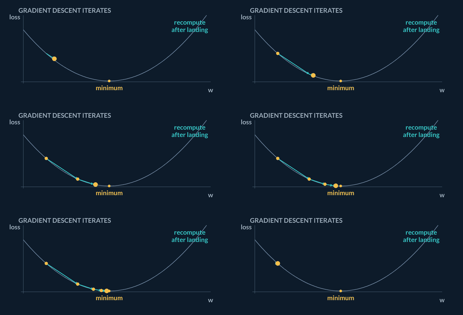
Animation: a U-shaped loss bowl with a gold dot moving from left to right toward the minimum. Each teal segment appears only after the dot lands, showing that the gradient is recomputed at the new point before the next shorter step. — Gradient descent is update, land, recompute, then update again. The arrows shrink because the local slope changes near the bottom of the loss bowl.

Iteration loop

StartCompute the gradient at w_t.
MoveSet w_{t+1}=w_t-\eta L'(w_t).
RefreshCompute L'(w_{t+1}) before another update.

Second step uses a smaller gradient

Continue the previous example with L(w)=(w-3)^2, w_1=2, and \eta=0.25.

L'(2)2(2-3)=-2
w_2=2-0.25(-2)2.5
L(2.5)0.25

Pro tip. The gradient magnitude fell from 4 to 2, so the second step is naturally smaller with the same learning rate.

After one step moves w, the next step should:

Recompute L'(w) at the new point
Reuse the first gradient forever
Set \eta=0
Ignore the objective

The local uphill direction changes as you move.

4Stopping uses progress, not a fixed ritual

Gradient descent is usually stopped when further updates are no longer buying meaningful improvement. A small gradient, a tiny loss change, or a validation-loss turn can all be stopping evidence.

The stopping rule should be tied to the objective. Running more steps is useful only while the score is still improving in a meaningful way.

Later arrows near the bottom of the bowl would be shorter and produce smaller loss drops.

Check a stopping signal

Measure gradientA small |L'(w)| suggests a flat region.
Measure loss changeCompare the loss before and after the latest step.
DecideStop only when the improvement is below the chosen tolerance.

Loss improvement is shrinking

For L(w)=(w-3)^2, compare the improvements from w=2 to 2.5 and from w=2.5 to 2.75.

L(2) and L(2.5)1 and 0.25
First improvement1-0.25=0.75
L(2.75)(2.75-3)^2=0.0625
Second improvement0.25-0.0625=0.1875

Pro tip. The optimizer is still improving, but the improvement is shrinking as the parameter nears the minimum.

A sensible stopping idea is:

Stop when loss/gradient progress stalls, not merely after a fixed ritual count
Always run exactly 100 steps
Stop when \eta is large
Stop when w becomes complex

Progress in the objective (or gradient norm) is the signal.

Notes

The gradient points in the direction of steepest local increase, so the negative gradient is the local decrease direction.
Gradient descent improves the objective by taking repeated small steps in that negative-gradient direction.
Each step uses the gradient at the current parameter value, then recomputes at the new value.

Formulas

\theta_{t+1}=\theta_t-\eta\nabla J(\theta_t).
For one parameter, w_{t+1}=w_t-\eta L'(w_t).

Exam traps & shortcuts

The sign matters: adding the gradient climbs the hill, subtracting it descends.
A gradient is local information, not a map of the whole loss surface.

Reference tables

These are the pieces that must be visible in a hand calculation.

One-step descent ledger
Piece	Example value	Role
Current parameter	w_0=1	Where the step begins
Gradient	L'(1)=-4	Local uphill direction
Learning rate	\eta=0.25	Scale of the step
New parameter	w_1=2	Result after subtracting \eta L'(w_0)

Recap

Gradient descent is calculus turned into an update loop.

Gradient: The gradient points locally uphill; the negative gradient is the descent direction.
Update: w_{t+1}=w_t-\eta L'(w_t) for a one-parameter objective.
Checked step: For L(w)=(w-3)^2, w_0=1, and \eta=0.25, one step gives w_1=2 and loss falls from 4 to 1.
Iterate: Recompute the gradient after every move; the old slope belongs to the old point.

Practise Gradient Descent

Reading is free and needs no account. Practice, mocks and progress live in the app.

A 5-question practice set that ends the chapter
4 quick checks with worked explanations
Timed mocks scored with the real marking scheme
Readiness tracked per topic, kept on your device

Continue with Google — freeNo card, no trial. Works offline once installed.