Engineering Mathematics · Optimization
Learning Rate
In Engineering Mathematics because even the right direction can fail if the step size is too timid or too aggressive.
Direction is only half of an optimization update. The learning rate controls how far the algorithm trusts the current gradient on each step.
- Engineering Mathematics
- Medium level
- 4 concepts
1The learning rate scales the gradient
The learning rate \eta multiplies the gradient before it is subtracted. With the same current point and the same gradient, changing \eta changes only the step length.
That makes learning-rate choice a numerical stability decision, not a change in the objective or in the gradient itself.
Figure. The learning rate scales the same gradient direction into a shorter or longer parameter step. Direction comes from the gradient; length comes from eta.
Same gradient, different steps
- Hold slope fixedStart from the same w_t and compute the same L'(w_t).
- Choose \etaMultiply that gradient by the learning rate.
- Compare movesThe sign is unchanged; only the distance changes.
Two step lengths from one gradient
For L(w)=(w-3)^2 at w=1, use the same gradient L'(1)=-4 with \eta=0.05 and \eta=0.25.
- \eta=0.05: w_1=1-0.05(-4)1.2
- L(1.2)(1.2-3)^2=3.24
- \eta=0.25: w_1=1-0.25(-4)2
- L(2)1
Pro tip. Both steps move downhill from loss 4, but \eta=0.25 uses the same slope more effectively than \eta=0.05 here.
Same gradient g=-4, compare \eta=0.05 vs 0.25 at w=1. Updates?
- \Delta w=+0.2 vs +1.0
- \Delta w=-0.2 vs -1.0
- Identical updates
- Only \eta=0.05 moves
\Delta w=-\eta g, so -0.05(-4)=0.2 and -0.25(-4)=1.
2Too large a learning rate can overshoot
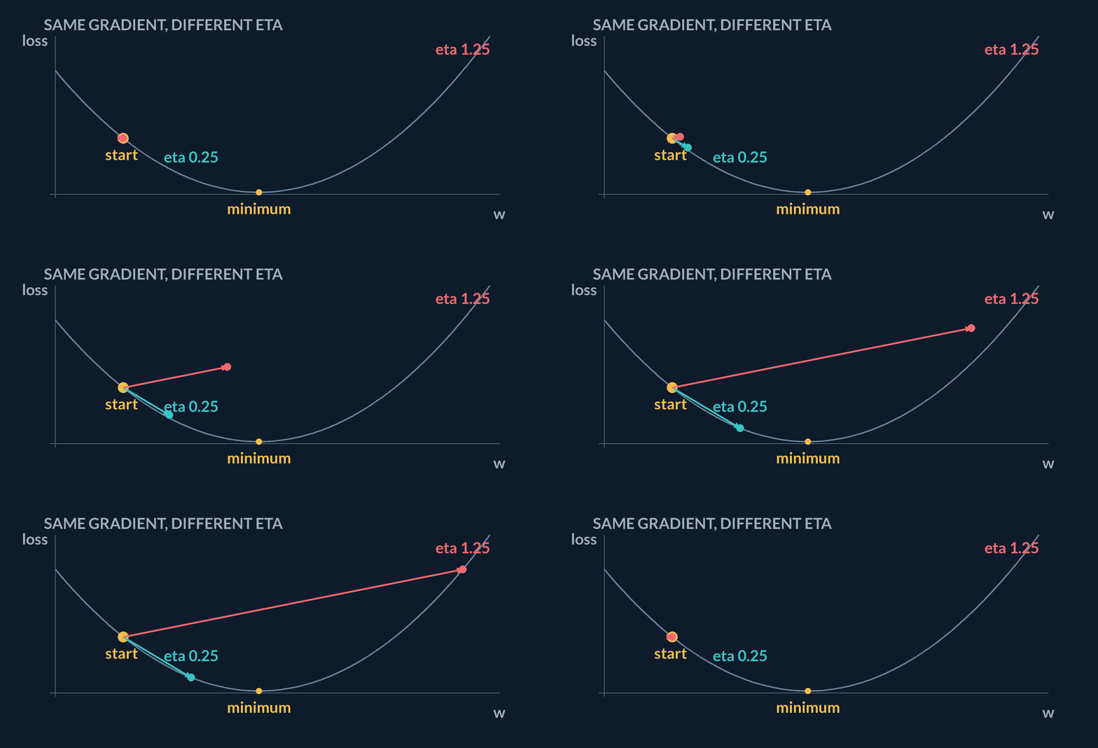
A descent direction is only locally reliable. If \eta is too large, the step can jump past the low region and land at a point with worse loss than before.
This failure can happen even when the gradient sign is correct; the step length is the problem.
Diagnose overshoot
- Use same gradientKeep L'(1)=-4 fixed.
- Try large \etaA large multiplier jumps far past the minimum.
- Check lossOvershoot is confirmed when the new loss is higher.
Progress versus overshoot from the same gradient
For L(w)=(w-3)^2 at w=1, compare \eta=0.25 and \eta=1.25 using the same gradient -4.
- Starting loss L(1)4
- \eta=0.25: w_1=1-0.25(-4)2, so L(2)=1
- \eta=1.25: w_1=1-1.25(-4)6, so L(6)=9
- Verdict\eta=0.25 progresses; \eta=1.25 overshoots and worsens loss
Pro tip. The overshoot example uses the same gradient. The bad outcome comes only from trusting that local slope too far.
Coding lab. Compare calm vs overshooting steps runs in the app, with checks on your output.
Too large \eta can:
- Jump past the minimum and increase loss
- Only slow convergence, never increase loss
- Delete the gradient
- Force bias to zero
Overshooting is the classic large-step failure mode.
3Loss history reveals step-size trouble
Training loss over time is often the first signal that \eta is wrong. Slow steady decline suggests a conservative learning rate; jumps or repeated increases suggest an aggressive one.
The symptom is not just whether the parameter moves a lot. What matters is whether the objective decreases reliably.
Figure. Loss history is a symptom chart: steady decrease suggests usable steps, while jumps and rebounds warn that the learning rate may be too large.
Read the history
- Slow declineLower loss each step, but only a little.
- OscillationLoss alternates across the low region.
- DivergenceLoss grows because steps keep landing farther away.
Two losses diagnose one step
A run starts at loss 4. One learning rate gives next loss 3.24; another gives next loss 9. Classify the symptoms.
- Loss change for 3.243.24-4=-0.76
- InterpretationProgress, but modest
- Loss change for 99-4=5
- InterpretationOvershoot or divergence warning
Pro tip. Tune \eta from the loss history. A dramatic parameter move is not useful if the objective climbs.
Loss sequence 4 \to 3.2 \to 2.6 vs 4 \to 9 \to 25 suggests:
- Stable decrease vs divergent/overshooting step size
- Both are healthy
- The second is always better
- Learning rate is unused in both
Monotone decrease looks healthy; explosion screams \eta too large.
4A simple quadratic shows the stability threshold
For L(w)=(w-3)^2, the update transforms the error e_t=w_t-3 into e_{t+1}=(1-2\eta)e_t. That factor says whether errors shrink, flip sign, or grow.
This threshold is special to this scaled quadratic, but the habit generalizes: inspect whether the update damps the error or amplifies it.
The stable case shortens the distance to w=3; the unstable case crosses the minimum and lands farther away.
Read the multiplier
- Derive errorSubstitute w_t=3+e_t into the update.
- Find factorThe next error is (1-2\eta)e_t.
- JudgeMagnitude below 1 shrinks; magnitude above 1 grows.
Why \eta=1.25 diverges here
Start at w=1, so e_0=-2. Compare the error multiplier for \eta=0.25 and \eta=1.25.
- \eta=0.251-2\eta=0.5
- Next error0.5(-2)=-1, so w_1=2
- \eta=1.251-2\eta=-1.5
- Next error-1.5(-2)=3, so w_1=6
Pro tip. The large learning rate not only flips across the minimum; it makes the error magnitude grow from 2 to 3.
For L(w)=\frac{1}{2}aw^2, updates stay stable only for sufficiently small \eta. This is about:
- A step-size limit set by curvature a
- Labels in the dataset
- Whether w is integer
- Batch size alone
Quadratic analysis yields |1-\eta a|<1 style thresholds.
Notes
- A small learning rate can make progress painfully slow.
- A large learning rate can overshoot, oscillate, or diverge because the local slope stops being a good guide too far away.
- The same gradient can produce progress or failure depending only on the learning rate.
Formulas
- The scalar \eta in \theta_{t+1}=\theta_t-\eta\nabla J(\theta_t) is the learning rate.
Exam traps & shortcuts
- Bad training dynamics are often a step-size problem before they are a model-design problem.
- Judge a learning rate by the loss after the step, not by how dramatic the parameter move looks.
Reference tables
All rows use L'(1)=-4 for L(w)=(w-3)^2.
| \eta | New w | New loss | Read |
|---|---|---|---|
| 0.05 | 1.2 | 3.24 | Slow progress |
| 0.25 | 2 | 1 | Good progress |
| 1.25 | 6 | 9 | Overshoot |
Recap
The learning rate decides how far one trusted gradient is allowed to move the parameter.
- Scale
- \eta scales the gradient before subtraction.
- Progress
- For L(w)=(w-3)^2 at w=1, \eta=0.25 gives w_1=2 and loss 1.
- Overshoot
- The same gradient with \eta=1.25 gives w_1=6 and loss 9, worse than the starting loss 4.
- Symptom
- Judge \eta by the loss history: slow decline, oscillation, or divergence.
Practise Learning Rate
Reading is free and needs no account. Practice, mocks and progress live in the app.
- A 5-question practice set that ends the chapter
- 4 quick checks with worked explanations
- Timed mocks scored with the real marking scheme
- Readiness tracked per topic, kept on your device