Statistical Inference · Statistical Inference
The sampling distribution
In Statistical Inference because the would-repeat picture — many weeks' means in one pile — is how we measure a sample's wobble.
Imagine the shop could replay the week. Each replay draws eight customers and writes one mean spent. Do that many times and the means form a pile. That pile is the sampling distribution of the sample mean — the picture of how the statistic moves when the sample is redrawn. Week 1's 220 is one dot in the pile, not the pile.
- Statistical Inference
- Medium level
- 5 concepts
1Replay the week
You cannot actually rewind the counter. You can still picture it: many weeks, each week eight people, each week a mean spent, each mean dropped as a dot onto a number line. The typical-week value stays put. The dots move, because each week is a new sample.
Week 1's 220 is one of those dots. In the picture we author, the pile sits around Rs 210. 220 is ordinary in that cloud — a few rupees off the centre, not a verdict. That is the point of replaying: one week stops looking like the shop.
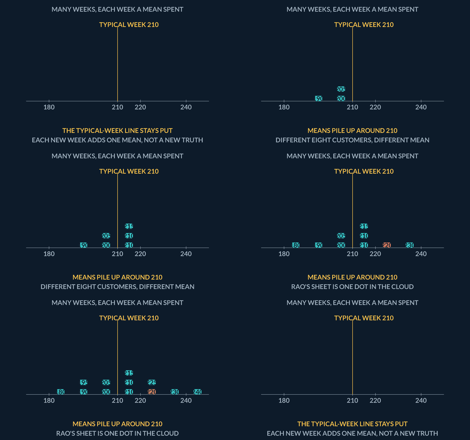
The replay
- Draw eight customersOne pretend week, one mean spent.
- Drop the meanA tile on the number line, not a new truth.
- RepeatThe pile of tiles is the sampling distribution.
Coding lab. Resample the week runs in the app, with checks on your output.
What hypothetical experiment forms the basis of a sampling distribution?
- Taking one sample and shuffling its feature columns 10,000 times
- Running gradient descent with 100 different learning rate initializations
- Repeatedly drawing samples of size n under identical conditions and recording each sample statistic
- Surveying the entire population repeatedly until variance becomes zero
The sampling distribution is the distribution of values a statistic would take if the sampling process were repeated infinitely.
2The pile of means
The pile of replayed means is the sampling distribution. It is a picture of a statistic, not of one customer. Anu's Rs 320 does not appear as a tile. Chitra's 510 does not either. The tiles are week means — 220, 225, and the other would-repeat numbers.
If the pile is tight, one week's mean is a stable story. If the pile is wide, one week's mean is a noisy story. We have not yet measured the width. We have named the object that has a width: the cloud of the sample mean, not the spread of people.
Figure. A sketch of the would-repeat pile: many week means sit near 210. Week 1's 220 is one of them.
| Object | In the pile? |
|---|---|
| A week mean | Yes — that is the statistic |
| Anu's Rs 320 | No — that is one person |
Coding lab. Centre of the pile runs in the app, with checks on your output.
What does each individual point in the sampling distribution of the mean represent?
- The individual spend value of a single customer row
- The residual error of a linear regression prediction
- The calculated mean of one full sample of n observations
- A discrete cluster centroid in k-means feature space
The sampling distribution is a distribution of a statistic (e.g. sample mean), not of raw individual data points.
3How much the mean wobbles
The eight spent values spread a lot: Deepak at 0, Chitra at 510. That spread of people is the standard deviation, about Rs 179. Call it s when it is computed from the sample. It answers how different two customers are — a person-to-person width.
The standard error answers a different question: how different two week-means are. Take 179 and divide by the square root of 8, because a week averages eight people. That is about Rs 63. The mean wobbles by tens of rupees, not by hundreds.
Keep the nouns: s is the spread of people. The standard error — SE — is the spread of the sample mean. The next interval is built from 63, not from 179.
Figure. The eight spent values spread a lot: Deepak at 0, Chitra at 510. That people-spread is s ≈ 179.4. The standard error is how week-means wobble: 179.4 / √8 = 63.4. Bars are to scale with those two lengths. Keep the nouns: s is people; SE is the mean.
From people-spread to mean-wobble
Week-1 spent values have sum of squared deviations 225400 from the mean 220. What is the standard error of the mean?
- 225400 / 732200
- sqrt(32200)179.4
- 179.4 / sqrt(8)63.4
Pro tip. 179.4 is how people differ. 63.4 is how week-means differ. Do not swap the nouns.
Coding lab. SD then SE runs in the app, with checks on your output.
What is the critical conceptual difference between standard deviation (s) and standard error (SE)?
- Standard deviation applies only to normal distributions while standard error applies to uniform distributions
- Standard deviation measures the spread of individual observations, while standard error measures the spread of sample statistics
- Standard error is always strictly larger than the sample standard deviation
- Standard deviation is computed from populations while standard error is computed from algorithms
Standard deviation s quantifies the dispersion of raw data points; standard error SE = s / sqrt(n) quantifies the uncertainty of the sample estimator.
4Four times the rows, half the wobble
The formula is SE = s / sqrt(n). s is still about 179, the people-spread. n is the number of customers in the sample. The n sits under a square root, so growing the sample calms the mean slowly. Four times as many customers halves the standard error, not quarters it.
From n = 8 to n = 32, SE goes from about 63 to about 32 if s stays near 179. That is why the owner cannot buy certainty with one extra row, and why thirty-two rows are meaningfully calmer than eight. The square root is the whole lesson in the formula.
Figure. SE at n = 8 is about 63. SE at n = 32 is about 32. Four times the rows halves the wobble.
Quadruple n
If s stays 179.4, what is SE at n = 8 and at n = 32?
- 179.4 / sqrt(8)63.4
- 179.4 / sqrt(32)31.7
Pro tip. 32 is 4 × 8, and 31.7 is about half of 63.4. The root is doing that.
Coding lab. SE at two n runs in the app, with checks on your output.
According to the formula SE = s / sqrt(n), what happens to the standard error if sample size n is quadrupled?
- The standard error is cut to one fourth of its original value
- The standard error doubles due to increased data volume
- The standard error is halved, reducing uncertainty by a factor of two
- The standard error remains completely unchanged
Because n is inside the square root (sqrt(4n) = 2*sqrt(n)), multiplying n by 4 divides SE by 2.
5SE is not the spread of people
Customers still differ by about Rs 179 whether you watch one week or many. Deepak can still spend 0 and Chitra 510. That SD does not shrink when n grows. What shrinks is the wobble of the average.
If you quote 179 as 'how unsure we are about the week mean', you have named the wrong width. The interval in the next lesson is built from 63, not from 179. People stay spread out. The mean calms down.
No diagram — the idea is carried by the prose, table, code block or coding lab.
| Width | Noun | Week-1 size |
|---|---|---|
| SD | How people differ | about 179 |
| SE | How week-means differ | about 63 |
Coding lab. Do not swap them runs in the app, with checks on your output.
The eight customers' spent values have SD about 179. The standard error of the mean is about 63. Which sentence is right?
- 63 is how much the week mean wobbles; 179 is how much people differ
- 179 is the chance the mean is wrong
- 63 is Deepak's spend
SE = s / sqrt(n). Different nouns.
Notes
- In Statistical Inference because the would-repeat picture — many weeks' means in one pile — is how we measure a sample's wobble.
- You cannot actually rewind the counter. You can still picture it: many weeks, each week a mean spent, each mean dropped onto a number line. The typical-week value stays put. The dots move.
- The pile of replayed means is the sampling distribution. It is a picture of a statistic, not of one customer. Anu's Rs 320 does not appear as a tile. The tiles are week means.
Exam traps & shortcuts
- A sample number describes these rows. A population claim reaches past them.
- Fail-to-reject is not proof. A p-value is not the chance the null is true.
Recap
The sampling distribution is the would-repeat pile of the statistic. Standard error is how wide that pile is — not how spread the eight people are.
- Replay the week
- You cannot actually rewind the counter. You can still picture it: many weeks, each week eight people, each week a mean spent, each mean dropped as a dot onto a number line. The typical-week value stays put. The dots move, because each week is a new sample.
- The pile of means
- The pile of replayed means is the sampling distribution. It is a picture of a statistic, not of one customer. Anu's Rs 320 does not appear as a tile. Chitra's 510 does not either. The tiles are week means — 220, 225, and the other would-repeat numbers.
- How much the mean wobbles
- The eight spent values spread a lot: Deepak at 0, Chitra at 510. That spread of people is the standard deviation, about Rs 179. Call it s when it is computed from the sample. It answers how different two customers are — a person-to-person width.
- Four times the rows, half the wobble
- The formula is SE = s / sqrt(n). s is still about 179, the people-spread. n is the number of customers in the sample. The n sits under a square root, so growing the sample calms the mean slowly. Four times as many customers halves the standard error, not quarters it.
Practise The sampling distribution
Reading is free and needs no account. Practice, mocks and progress live in the app.
- A 3-question practice set that ends the chapter
- 5 quick checks with worked explanations
- Timed mocks scored with the real marking scheme
- Readiness tracked per topic, kept on your device