Artificial Intelligence · AI Foundations
A* Search
In AI because A* is the workhorse of optimal planning — the guided-search algorithm robotics stacks, game engines and interview questions all reach for.
Heuristics and their guarantees are in hand; this lesson builds the algorithm that spends them. A* ranks its frontier by f = g + h and, with the properties of the last lesson, returns a cheapest path while expanding less of the graph than uniform-cost search. The load-bearing details — goal-test on pop, what each term of f buys, why stopping is safe — are exactly where implementations and interviews go wrong.
- Artificial Intelligence
- Medium level
- 5 concepts
1The algorithm
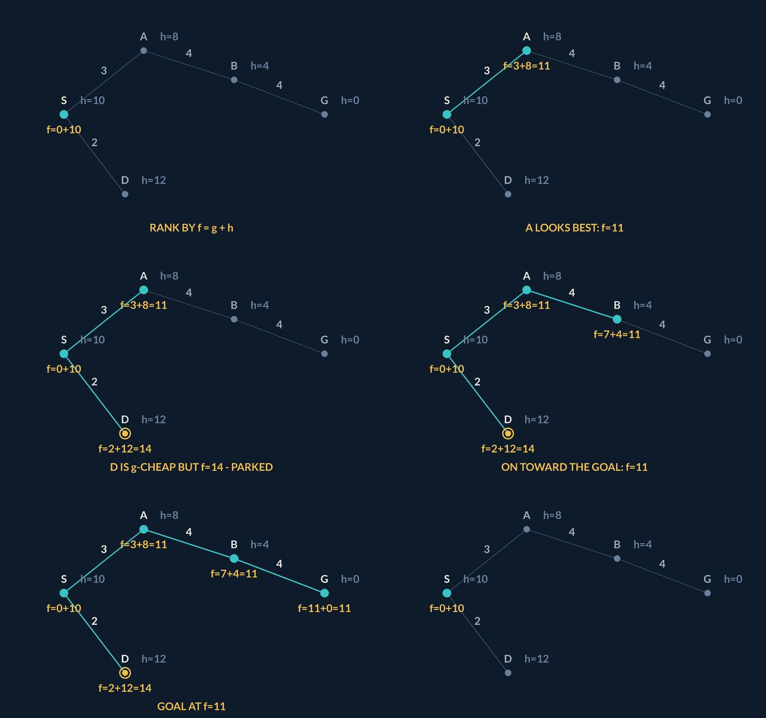
A* keeps a frontier ordered by f(n) = g(n) + h(n): g is the cheapest cost found so far from the start to n, h is the heuristic's estimate of what remains, so f is an optimistic forecast of the best total cost of any solution passing through n. The loop is short — pop the smallest f, stop if it is a goal, otherwise expand it: compute each successor's g, and insert or update it on the frontier.
The forecast is what buys focus. A node reached cheaply but pointing away from the goal carries a small g and a large h, and its f sinks it down the queue: in the animation, the decoy D is generated at f = 2 + 12 = 14 and simply never expanded while the real contenders open at 11. Strip h away and that focus vanishes — with h = 0 everywhere, A* is uniform-cost search.
An implementation is a binary heap keyed by f, a table of the best g known per node, and parent pointers to rebuild the path at the end. Time is dominated by heap operations, but the binding constraint in practice is memory: the frontier of a hard instance can approach the size of the reachable graph, which is why memory-bounded variants such as IDA* exist.
A* on the graph from the cost-aware lesson
Same weighted graph as uniform-cost search used: S→A 2, A→G 9, S→B 5, B→G 3, direct S→G 10 — now with the admissible estimates h(S) = 7, h(A) = 8, h(B) = 3, h(G) = 0.
- Expand S: f(A) = 2 + 8, f(B) = 5 + 3, f(G) = 10 + 010, 8, 10
- Smallest f pops: B at 8, generating G via B at f = 8 + 08
- G pops at f = 8path S→B→G, cost 8
- Expansions S, B, G — against S, A, B, G for uniform-costsame optimal path, one expansion fewer
Pro tip. h(A) = 8 is what parked the A branch: its forecast of 10 never became the cheapest thing waiting. Uniform-cost search, with no forecast, paid to expand A at g = 2 before it ever reached B.
Coding lab. Implement A* on the lesson graph runs in the app, with checks on your output.
2Goal-test on pop, not on generation
There are two moments an implementation can ask whether a node is the goal: when it is first generated as a successor, or when it is popped off the frontier. Correct A* tests when it is popped, not when it is generated — and the difference is not pedantry, it is the optimality guarantee.
At generation time a node carries whatever g the discovering route happened to have; nothing certifies that route as the cheapest. Only when the node's f is the smallest thing on the frontier is the certificate issued — that is the moment the stopping argument applies. Dijkstra's algorithm has exactly the same rule, and porting it wrongly is the single most common A* implementation bug.
The lesson graph fails loudly under the wrong test: the direct S→G edge generates the goal during the very first expansion, at cost 10. Accept it there and the search never learns that S→B→G finishes at 8.
Figure. Expanding S generates G on the direct edge at g = 10. Accept the goal at generation and the search returns 10. Test at pop and B pops first; G via B waits, then pops at 8 — S→B→G.
Where the certificate comes from
- GeneratedA successor arrives carrying the g of whichever route found it — possibly a poor one.
- WaitingOn the frontier its f competes; cheaper routes into the same node may still replace its g.
- PoppedSmallest f anywhere: no waiting path can undercut it, so the goal test is now safe.
The 10 the wrong test returns
Run A* on the lesson graph (S→A 2, A→G 9, S→B 5, B→G 3, S→G 10; h = 7, 8, 3, 0) but accept the goal at generation instead of at pop.
- Test at generation — expanding S produces G with g = 10accepted immediately: returns cost 10
- Test at pop — B pops first at f = 8, generating G via B at f = 8G waits on the frontier
- G pops with the smallest freturns S→B→G, cost 8
- Price of the early test: 10 against 825% dearer, reported as if optimal
Pro tip. The buggy version terminates normally and returns a legal path — nothing crashes. Wrong-goal-test A* is only caught by checking its answers against a known optimum, which is one reason the small hand-checkable graph is worth keeping around.
3What g and h each buy you
The two terms of f audit different things. g is the meter: cost actually paid from the start, so no forecast can hide a dear route already taken. h is the compass: where the remaining cost probably lies, so effort bends toward the goal instead of flooding outward evenly.
Delete either term and the algorithm degenerates into something with its own name. Setting h = 0 leaves f = g, which is uniform-cost search — still optimal, completely blind, expansion counts balloon. Dropping g leaves f = h, which is greedy best-first search — fast when the compass is good and unprotected when it lies, as the next concept demonstrates.
Between the poles lies a dial rather than a switch. Weighted A* ranks by f(n) = g(n) + w \cdot h(n) with w > 1, deliberately over-trusting the compass: it expands fewer nodes and returns a path guaranteed to cost at most w times the optimum when h is admissible. Production planners run it with w chosen on purpose; the defect is only ever in turning the dial without knowing.
Figure. The frontier the moment S is expanded, each bar an f-value: paid cost stacked under forecast remainder. Reading g alone chases 'via A' (2 paid); reading h alone pops the direct goal (0 left) and returns the dear 10; only the sum — shortest overall bar, via B at 8 — is protected in general.
| Ranking | Algorithm | Promise |
|---|---|---|
| f = g | Uniform-cost search | Optimal; expands in every direction |
| f = h | Greedy best-first | No optimality; exactly as good as the compass |
| f = g + h | A* | Optimal with admissible h (consistent, for graph search) |
| f = g + w·h, w > 1 | Weighted A* | Cost at most w × optimum; fewer expansions |
You set h to zero at every node. What algorithm are you now running?
- Greedy best-first search, because the estimate no longer competes with the path cost
- Depth-first search, because nothing pulls the search toward the goal any more
- An inadmissible A*, because zero understates every remaining cost
- Uniform-cost search, because the ranking has nothing left in it but the cost already paid
f = g + h with h gone is f = g, which is exactly cheapest-path-so-far. Note that zero never overestimates, so this degenerate heuristic is perfectly admissible.
4Greedy best-first, and when it fails
Greedy best-first search ranks the frontier by h alone: always expand whatever looks nearest the goal. It follows the compass and never reads the meter, so cost already sunk into a path counts for nothing.
That is exploitable by construction. Give S two roads: through X, costing 2 then 2, and through Y, costing 1 and then a 20-cost cliff. Set h(X) = 2 and h(Y) = 1 — both admissible, since the true remainders are 2 and 20. Greedy compares 1 against 2, dives through Y, meets the goal and returns a cost-21 path. The admissibility of both estimates protected nothing, because greedy never asks what has been paid.
A* on the same instance also tries Y first — f(Y) = 2 beats f(X) = 4 — but the cliff surfaces in g: the goal via Y waits at f = 21 while X pops at 4 and delivers the goal at f = 4. Optimism misleads both algorithms for a step; only the one carrying g recovers. Greedy earns its keep where h is excellent and any path will do — and in interviews, as the standard demonstration that an admissible heuristic does not make every search optimal.
Figure. The upper road through X costs 4 in total; the lower road through Y looks nearer (h = 1 against 2) and hides a 20-cost edge behind its first cheap step. Ranking by h alone commits to Y and never revisits the choice; carrying g lets the 20 surface before an answer is returned.
The compass without the meter
S→X 2, X→G 2; S→Y 1, Y→G 20. Estimates h(X) = 2, h(Y) = 1, h(G) = 0 — both admissible, since the true remainders are 2 and 20.
- Greedy from S: h(Y) = 1 < h(X) = 2expand Y
- Y's successor G carries h = 0returns S→Y→G, cost 1 + 20 = 21
- A* instead: f(Y) = 1 + 1, f(X) = 2 + 22 and 4 — Y still pops first
- G via Y waits at f = 21; X pops at 4, G via X at f = 4returns S→X→G, cost 4
- Greedy's path against the optimum: 21 / 45.25× dearer
Pro tip. Notice what failed and what did not: h was admissible throughout. The guarantee A* enjoys is a property of using g and h together, not of the heuristic alone.
5Why the first goal pop is optimal
The theorem, stated the way an exam wants it: tree-search A* with an admissible heuristic is cost-optimal; graph-search A* is cost-optimal when the heuristic is consistent, or when inconsistency is repaired by reopening. Write C^* for the cost of an optimal solution.
The argument has two halves. First, some prefix of an optimal path is always sitting on the frontier, and admissibility keeps that entry's f at or below C^* — the estimate never overstates what the rest of that optimal path costs. Second, A* pops lowest f, and at a goal h is zero, so a popped goal's f equals the genuine cost of the path being returned. Pop a goal dearer than C^* and the two halves collide: the optimal prefix, waiting at f at most C^*, was strictly cheaper and would have popped first.
Each hypothesis is load-bearing, and the neighbouring lessons are what happens when one is removed. Overestimating h buries the optimal prefix behind an inflated f — the bad-heuristics concept runs those numbers. Inconsistency in graph search lets a node settle on a stale g — the reopening concept. And testing the goal at generation reads f before the certificate exists. The proof is short precisely because the definitions were built to make it short.
Figure. At the instant a goal reaches the front, its f is the fully-paid path cost (h = 0). A prefix of an optimal path is still waiting with f ≤ C* by admissibility. A goal popping above C* would mean that cheaper prefix was passed over — impossible under lowest-f-first.
The stopping argument, in order
- Prefix on frontierSome node of an optimal path is always waiting, with f ≤ C* by admissibility.
- Goal pops honestAt a goal h = 0, so its f is the true, fully-paid cost of the path about to be returned.
- ContradictionA goal popping above C* would mean the cheaper optimal prefix was passed over — impossible under lowest-f-first.
A* pops the goal from the frontier. Why is it safe to stop rather than keep looking for something cheaper?
- The goal is always the last node A* generates
- h is zero at the goal, so no better estimate can exist
- It is not safe: A* has to drain the frontier before it can report a path
- Every path still waiting already carries an f-value at least as large, and h never overstates what is left, so none of them can finish cheaper
The stopping argument needs both halves. Cheapest-f-first means everything waiting looks at least as expensive, and admissibility means those f-values are not flattering.
Notes
- A* orders its frontier by f(n) = g(n) + h(n) and always expands the smallest forecast first.
- Goal-test when a node is popped, not when it is generated — only the pop certifies the cheapest route.
- Tree-search A* is optimal with an admissible heuristic; graph search needs consistency or reopening.
Formulas
- f(n) = g(n) + h(n): cost paid so far plus estimated remainder
- Weighted A*: f(n) = g(n) + w · h(n) with w > 1 returns a path costing at most w × the optimum
Exam traps & shortcuts
- Goal-test when a node is popped, never when it is generated — the generation-time test returns the first route found, not the cheapest.
- If A* expands nearly as many nodes as uniform-cost search, h is adding almost nothing — measure expansions, not wall-clock time, when judging a heuristic.
- A* is memory-bound long before it is time-bound: the frontier of a hard instance can approach the size of the reachable graph.
Recap
This lesson in brief:
- The rule
- A* expands the smallest f = g + h: cost paid plus estimated remainder, an optimistic forecast of the total.
- The goal test
- Test at pop, never at generation — only the pop certifies that no waiting route is cheaper.
- g and h
- g is the meter, h the compass: h = 0 gives uniform-cost search, dropping g gives greedy best-first, and w·h with w > 1 trades optimality for speed with a w × optimum bound.
- Optimality
- With admissible h (consistent, for graph search) the first goal popped is a cheapest solution — the optimal prefix waiting at f ≤ C* makes anything dearer impossible.
Practise A* Search
Reading is free and needs no account. Practice, mocks and progress live in the app.
- 2 quick checks with worked explanations
- Timed mocks scored with the real marking scheme
- Readiness tracked per topic, kept on your device