Machine Learning · Machine Learning Core
Confusion Matrix
Name the four cells of a binary classifier — TP, FP, TN, FN — then compute and heat-map them on an imbalanced hold-out in the browser.
Before precision, recall or ROC, lock the four cells. This lesson names true positives, false positives, true negatives and false negatives, then lets you print rates and heat-map the same hold-out predictions in the browser.
- Machine Learning
- Medium level
- 5 concepts
- 10 practice questions
1Four outcomes, four names
Picture a bank's fraud detector. Every time a card payment comes in, a model looks at it and gives a yes-or-no answer: "I think this payment is fraud" or "I think this payment is legitimate." That answer is the model's prediction. But every payment also has a true answer — it really was fraud, or it really was legitimate — which the bank finds out later, for example when a customer disputes a charge. So for every single payment there are two facts side by side: what actually happened (the truth) and what the model said (the prediction). Sometimes the two agree, and sometimes they do not.
Because the truth has two possible values (fraud or legit) and the prediction has two possible values (fraud or legit), every payment lands in exactly one of 2 \times 2 = 4 possible outcomes. Each of the four has a name, and each name is worth a small story. A true positive (TP) is a payment that really was fraud and that the model also flagged as fraud — the thief got caught. A false negative (FN) is a payment that really was fraud but that the model waved through as legit — a missed alarm, and the thief walked away with the money.
The other two outcomes happen on legitimate payments. A false positive (FP) is a payment that was actually legit but that the model flagged as fraud — a false alarm, and an innocent customer gets their card blocked at the checkout. A true negative (TN) is a payment that was legit and that the model correctly let through — nothing happened, which is exactly what should happen. Notice the naming pattern: "positive" or "negative" describes what the model said (flagged or not flagged), and "true" or "false" says whether the model was right about it.
| Cell | Meaning |
|---|---|
| True positive | Positive label, predicted positive |
| False positive | Negative label, predicted positive |
| True negative | Negative label, predicted negative |
| False negative | Positive label, predicted negative |
A security scanner flags a benign visitor as an intruder. In the confusion matrix, this event is a:
- False Negative, because an intruder was missed by security
- False Positive, because the model made a positive call that was incorrect
- True Negative, because the visitor was indeed benign
- True Positive, because an alarm was successfully triggered
The call was positive (alarm flagged), but the truth was negative (benign visitor). Hence, a False Positive.
2Rows are truth, columns are the call
Now the general concept. Take a pile of test payments, sort every one of them into its outcome, and count how many landed in each. Arrange those four counts in a small two-by-two table and you have a confusion matrix. The name is literal: the table shows you exactly where the model is confusing one class with the other. In this course's layout, the rows of the table are the truth — the top row holds everything that was actually fraud, the bottom row everything that was actually legit — and the columns are the model's prediction, one column for "model said fraud" and one for "model said legit."
That orientation matters enough to say again. To find the right cell for a payment, ask two questions in order: first, what actually happened? That picks the row, because rows are the truth. Second, what did the model say? That picks the column, because columns are the prediction. A word of caution: not every textbook or library arranges it the same way — some swap rows and columns — so before you read any confusion matrix, check its axis labels and confirm which side is truth and which side is the model's call. Reading a flipped matrix silently swaps your missed alarms and your false alarms.
Figure. Rows are the truth, columns are the model's call, and every prediction lands in exactly one cell. The two green cells are agreement; the two red cells are the different ways to be wrong - a missed alarm (FN) and a false alarm (FP) - and every precision/recall story is an argument about which red cell hurts more.
| Truth (picks the row) | Model's call (picks the column) | Cell | Of the twelve payments |
|---|---|---|---|
| Fraud | Flagged | TP — hit | 3 (P1, P6, P9) |
| Fraud | Passed | FN — missed alarm | 1 (P4) |
| Legit | Flagged | FP — false alarm | 2 (P3, P11) |
| Legit | Passed | TN — correct pass | 6 (the remaining passes) |
Twelve payments, sorted by hand
The fraud desk pulls twelve card payments whose true labels are now known — the customers have confirmed which ones were really fraud — together with what the model said at the time. Each entry below reads (truth, model call): P1 (fraud, flagged), P2 (legit, passed), P3 (legit, flagged), P4 (fraud, passed), P5 (legit, passed), P6 (fraud, flagged), P7 (legit, passed), P8 (legit, passed), P9 (fraud, flagged), P10 (legit, passed), P11 (legit, flagged), P12 (legit, passed). Sort every payment into exactly one of the four cells and fill in TP, FN, FP and TN.
- Row question first — which payments were actually fraud? Scan only the truth entries: P1, P4, P6, P94 payments on the fraud row
- Column question for that row — of P1, P4, P6, P9, which did the model flag? P1, P6, P9 flagged; P4 was passedTP = 3, FN = 1
- The other eight payments were actually legit: P2, P3, P5, P7, P8, P10, P11, P128 payments on the legit row
- Column question again — of those eight, which did the model flag? P3 and P11 flagged; the other six passedFP = 2, TN = 6
- Every payment lands in exactly one cell, so the four counts must return the twelve rows: 3 + 1 + 2 + 612 — nothing dropped, nothing counted twice
Pro tip. The classic slip is to sort by the model's call first — collecting all five flagged payments into one pile. That pile mixes real frauds caught (TP) with innocent customers blocked (FP), which are opposite outcomes for the business. Always ask the questions in the concept's order: truth picks the row, then the call picks the column. And note P4 against P3: a missed fraud is a false negative because "negative" names what the model said (passed), while "false" says the model was wrong about it.
With rows as actual class and columns as the model's call, where does a real positive that the model predicted negative land?
- False positive — the model made a false call
- False negative — positive row, negative column
- True negative — the prediction was negative
- True positive — the row was truly positive
Name the cell from both coordinates: the truth is positive (row), the call is negative (column) — a missed positive, the false-negative cell.
3Every metric is a ratio of cells
Why go to this trouble instead of just quoting one score? Because every metric you will meet later — precision, recall, and the rest — is nothing more than a ratio built from these four counts. Precision is TP/(TP+FP): of everything the model flagged, how much was really fraud? Recall is TP/(TP+FN): of all the real fraud, how much did the model catch? If you cannot point at the cell that hurts your business — blocked customers live in FP, stolen money lives in FN — you have no basis for choosing which metric to care about.
The matrix is also where you watch a trade-off that no single number shows. Most classifiers actually produce a score, like "73% chance this is fraud," and a threshold decides how suspicious a payment must be before it gets flagged. Lower the threshold and the model flags more payments: some missed frauds move from the FN cell into the TP cell (good), but some clean payments move from the TN cell into the FP cell (bad). Raise the threshold and the traffic flows the other way. The four cells let you see exactly how much of each you are trading.
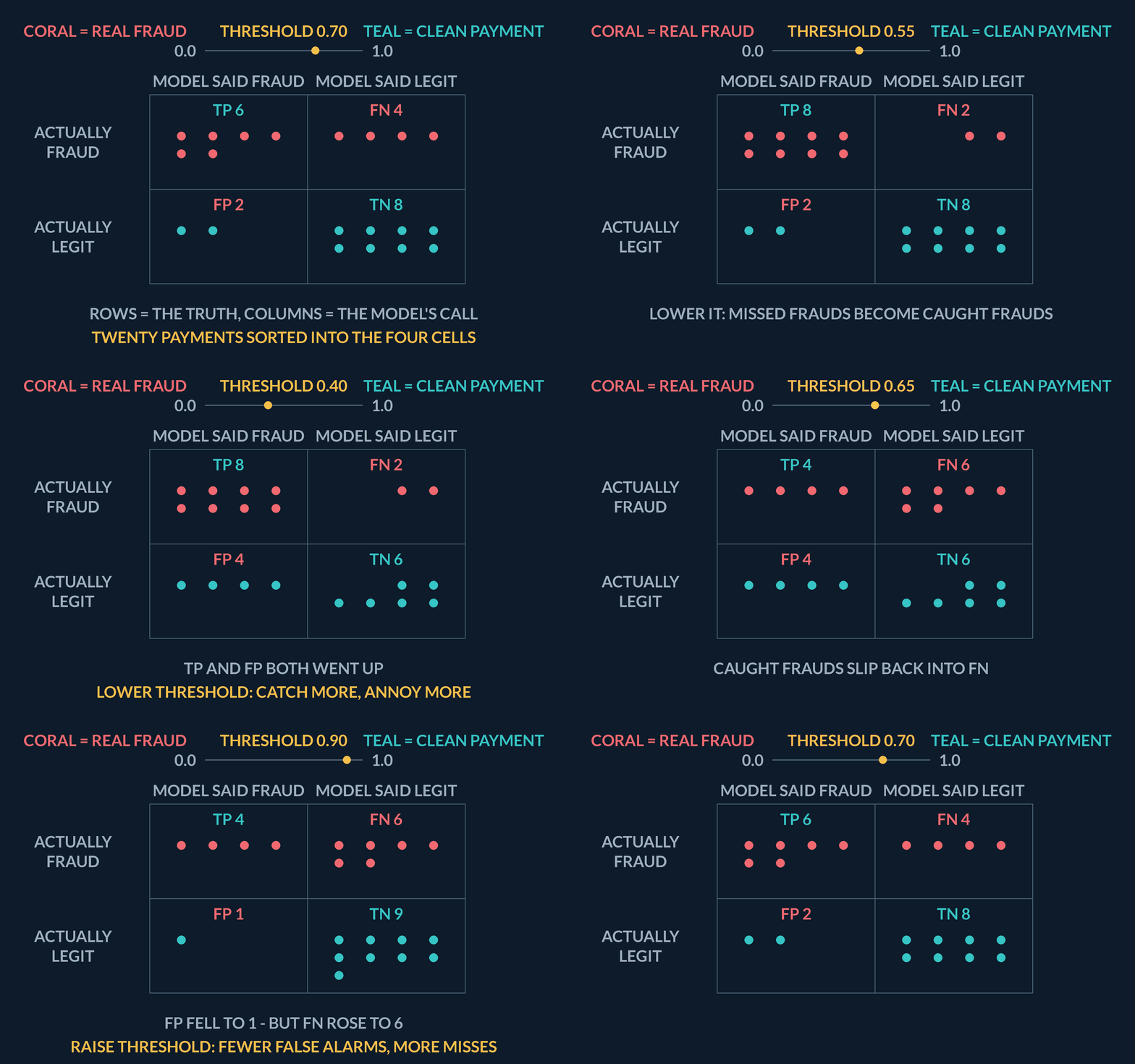
- Lay out the gridRows are actual class, columns are predicted — four cells: TP, FP, TN, FN.
- Read each cellTP and TN are correct; FP is a false alarm; FN is a missed positive.
- Derive ratesPrecision = TP/(TP+FP); recall = TP/(TP+FN) — each cell feeds both.
| Rate | Ratio of cells | Question it answers | Fraud matrix: TP 8, FP 3, FN 2, TN 87 |
|---|---|---|---|
| Precision | TP/(TP+FP) | Of everything flagged, how much was really fraud? FP is the blocked customer | 8/(8+3) \approx 0.727 |
| Recall | TP/(TP+FN) | Of all the real fraud, how much was caught? FN is the stolen money | 8/(8+2) = 0.80 |
| Accuracy | (TP+TN)/\text{total} | How many calls were right overall — high here because legit dominates | (8+87)/100 = 0.95 |
Three rates from the same four cells
Take the twelve payments the fraud desk already sorted: TP = 3 real frauds caught, FN = 1 fraud missed, FP = 2 innocent customers wrongly flagged, TN = 6 legit payments correctly left alone. Every metric is a ratio of these cells, so build three of them by hand. For each rate, first assemble its denominator from the cells — the pile the question is asked about — and only then divide: precision (of everything flagged, how much was really fraud?), recall (of all the real fraud, how much was caught?), and accuracy (of all twelve payments, how many calls were right?).
- Precision's pile is everything the model flagged, right or wrong: TP + FP = 3 + 25 flagged payments
- Precision, the real frauds among the flags: 3/50.6 — two of every five flags blocked an innocent customer
- Recall's pile is all the real fraud, caught or not: TP + FN = 3 + 14 real frauds
- Recall, the caught share of the real fraud: 3/40.75 — one thief in four walked away
- Accuracy's pile is all twelve payments, and its correct calls are both diagonal cells: (TP + TN)/12 = (3 + 6)/129/12 = 0.75
- Now read what each rate ignored: precision never touched the FN = 1 missed fraud, recall never touched the FP = 2 blocked customers, and only accuracy touched TNeach metric leaves cells out — that is why the desk needs more than one
Pro tip. Recall and accuracy both landed on 0.75 here, and they still answer different questions: 0.75 of the 4 real frauds were caught, while 0.75 of all 12 calls were right. A rate is a fraction of some pile, and the pile is named by the denominator you assembled first. Before comparing two rates — or celebrating that two agree — say out loud what each one is a fraction of.
Which confusion matrix cells are used in the denominator when calculating Precision?
- TP + FN, the total number of actual positive cases in reality
- TP + FP, the total number of instances the model predicted as positive
- TN + FP, the total number of actual negative cases in reality
- TP + TN + FP + FN, the entire dataset population
Precision answers 'Of all positive predictions made (TP + FP), how many were correct (TP)?'
4The accuracy trap
One last warning before you trust any headline number. Suppose only 2 of 100 payments are fraud, and a lazy model simply says "legit" every single time. It is right on 98 of the 100 payments, so its accuracy is 98% — and it has never caught a single fraud, because its TP cell is zero and both real frauds sit in the FN cell. Accuracy looked excellent while the model did nothing useful. The confusion matrix is the antidote: read the four cells before you quote any single rate.
Figure. A lazy model that answers legit every single time is right on 98 of the 100 payments, so its accuracy is 98% - and it has never caught a fraud: its TP cell is zero and both real frauds sit in the FN cell. Read the four cells before you quote any single rate.
Fill the do-nothing model's four cells
Take the lazy model from the prose at face value and audit it with the matrix. The batch is 100 payments, of which 2 really are fraud and 98 really are legit, and the model says "legit" every single time — it never flags anything. Fill in all four cells (remember: truth picks the row, the model's call picks the column), check the cells return all 100 payments, then compute the headline accuracy from the cells and, beside it, the recall — the share of real fraud this model caught.
- Fraud row first: both real frauds were waved through as legit, so nothing sits in the caught cellTP = 0, FN = 2
- Legit row: all 98 legit payments were also called legit, and nothing was ever flaggedFP = 0, TN = 98
- Cell check — the four counts must return the whole batch: 0 + 2 + 0 + 98100 — nothing dropped
- Accuracy from the cells, correct calls over all calls: (TP + TN)/100 = (0 + 98)/1000.98 — the shiny 98% headline
- Recall from the cells, frauds caught over real frauds: TP/(TP + FN) = 0/(0 + 2)0 — not one fraud caught
Pro tip. Try to compute this model's precision and the arithmetic itself refuses: TP/(TP+FP) = 0/0, a division with no answer, because the flagged pile is empty and there is nothing to grade. A metric that breaks is a message — the model never made a single positive call — and it is one more thing the 98% headline hid until the four cells were on the table.
In a medical diagnostic test where missing a fatal disease is disastrous, why is confusion matrix inspection necessary over accuracy?
- Because confusion matrices automatically adjust the classifier's decision threshold
- Because accuracy is mathematically undefined whenever false positives occur
- Because confusion matrices can only be generated for continuous regression outputs
- Because accuracy treats false negatives and false positives identically, hiding critical missed diagnoses
A false negative (missed fatal disease) has vastly higher real-world cost than a false positive (follow-up test). The confusion matrix reveals this critical breakdown.
5Lab: confusion matrix on an imbalanced set
This lab makes the four cells appear from real code instead of a story. You will build a small pretend dataset where the positive class is deliberately rare — about 1 row in 10 is positive, just like fraud is rare among payments; this is what "imbalanced" means. You then split the rows into a training set (which the model learns from) and a held-out test set (which the model never sees during learning), fit a classifier, and ask it to predict on the test rows. That gives you two arrays with matching lengths: `y_test`, the true label of every test row, and `pred`, the model's call for the same rows, in the same order. Those two arrays are all a confusion matrix needs.
Cell 1 fits the model and prints three scores: accuracy (the fraction of all test rows the model got right), precision (of the rows it flagged positive, how many really were), and recall (of the rows that really were positive, how many it caught). Watch the printed numbers carefully: on an imbalanced set it is completely normal to see a high accuracy sitting right next to a weak recall. That is the accuracy trap from the vocabulary concept happening live — the model can be "mostly right" simply by leaning on the huge negative class while missing many of the rare positives.
Cell 2 turns the same two arrays into a picture. The `confusion_matrix` function counts the four cells from `y_test` and `pred`, and `imshow` draws those counts as a heat-map — a colored grid where a darker square means a bigger count. The number printed inside each square is the actual count, so you can read TP, FP, FN and TN straight off the plot. This works without re-fitting anything because both cells run in one shared kernel: the variables Cell 1 created (`y_test` and `pred`) stay alive in memory, and Cell 2 simply reuses them. Try changing the colormap in Cell 2 and re-running only that cell — the counts stay identical, because nothing about the model changed.
The point to take away: the three printed rates and the heat-map are not different information. They are one set of four counts, viewed two ways. When a single score looks suspicious — and on imbalanced data it often should — the matrix is where you go to see which cell is really carrying the damage.
No diagram — the matrix is drawn by the coding lab plot, not a static figure.
| Step | Why |
|---|---|
| Hold out a test fold | Scores and the matrix must use rows the fit never saw |
| Print accuracy / precision / recall | Rates alone hide which cell is hurting |
| Heat-map y_test vs pred | Shared kernel: same arrays, four cells visible |
Coding lab. Confusion matrix on an imbalanced set runs in the app, with checks on your output.
In the lab, accuracy prints 0.94 but recall prints 0.20 on the imbalanced hold-out. Which picture does the heat-map show?
- A nearly diagonal matrix with all four cells balanced
- A heavy true-negative cell and most real positives sitting in the false-negative cell
- A heavy false-positive cell from over-flagging
- An empty true-negative cell — negatives were all missed
With rare positives, calling almost everything negative keeps accuracy high while the positives pile up as false negatives — the matrix makes that visible where the headline rate hides it.
Notes
- A binary classifier has four cells: true positives, false positives, true negatives, and false negatives.
- Rows are usually truth and columns the model's call — read the matrix before trusting any derived rate.
- Every precision and recall story is a story about those four counts.
Exam traps & shortcuts
- Keep lab datasets under 2000 rows in the browser runtime.
- Split train and test before fitting any model that sees labels.
Recap
This lesson in brief:
- Four cells
- A binary classifier has four cells: true positives, false positives, true negatives, and false negatives.
- Read before rates
- Rows are usually truth and columns the model's call — read the matrix before trusting any derived rate.
- Accuracy trap
- Accuracy alone can look fine on an imbalanced set while the matrix shows every positive was missed — read the four cells before quoting a headline rate.
Practise Confusion Matrix
Reading is free and needs no account. Practice, mocks and progress live in the app.
- 10 exam-style questions on this topic, with explanations
- A 5-question practice set that ends the chapter
- Timed mocks scored with the real marking scheme
- Readiness tracked per topic, kept on your device