Machine Learning · Machine Learning Core
Logistic Regression
Turn a linear score into a class probability with a sigmoid — the classification baseline after you have fitted a line for continuous targets.
Last lesson a straight line priced a flat — ₹7,900, a number on an open scale. Walk into a bank and the question changes: will this applicant repay, yes or no? Feed that question to the line and it happily outputs numbers like -4, 0.1 or +7, none of which is a yes or a no. This lesson fixes the ending: one S-shaped curve, the sigmoid, squashes any score into a probability between 0 and 1, and a threshold turns that probability into a decision. Then you fit a tiny logistic baseline and paint its decision regions in the browser.
- Machine Learning
- Medium level
- 4 concepts
- 10 practice questions
1Logistic regression
Picture a bank officer looking at a loan application. She has two facts in front of her: the applicant's monthly income and their existing debt. Her question is not "how much?" of anything — it is "will this person repay, yes or no?" A question whose answer is one of two categories (repay / default, spam / not spam, sick / healthy) is called a classification problem. Compare it with the last lesson: the rent was a number on an open scale — any rupee amount could come out. Here the answer can only land in one of two boxes. That one change — a category instead of a number — is the whole reason this lesson exists, and logistic regression is the standard first model for it.
Here is the surprise: logistic regression is the same weighted sum you already know from the rent line, with a new ending bolted on. It starts exactly like linear regression, computing a score z = w \cdot x + b. Unpack every symbol in that formula. x is the applicant's list of feature values — say income and debt, the numbers the bank actually knows. w is a list of weights, one per feature, that the model learns during training; each weight says how strongly that feature pushes the score up or down (debt would get a weight that pushes toward "default"). The dot w \cdot x means "multiply each feature by its weight and add the results up" — one combined number. b is the bias, a learned starting value the weighted sum gets added to, so the score is not forced to be zero when all features are zero. The result z is a single plain number that can land anywhere: -4, 0.1, +7, anything. It is not a probability yet — the sigmoid, next, is the new ending.
Figure. The start is pure linear regression: each feature the bank knows (income, debt) is multiplied by its learned weight, the results are added up with the bias b, and out comes a single plain number z that can land anywhere — -4, 0.1, +7.
| Symbol | What it is | In the loan example |
|---|---|---|
| x | The row's feature values | The applicant's income and debt — the numbers the bank actually knows |
| w | Learned weights, one per feature, pushing the score up or down | Debt gets a weight that pushes toward "default" |
| w \cdot x | Multiply each feature by its weight, add the results up | One combined number from income and debt |
| b | Learned bias the weighted sum is added to | Keeps the score from being forced to 0 when all features are 0 |
| z | One plain number, can land anywhere | -4, 0.1, +7 — not yet a probability |
Two applicants, two raw scores — by hand
The bank's fitted model uses the two features the officer has on file — monthly income and existing debt, both in thousands of rupees. Its learned numbers: weight -0.04 on income (every extra thousand earned pushes the score down, away from default), weight +0.09 on debt (every extra thousand owed pushes it up, toward default), and bias b = 0.5. Two new applicants walk in: applicant C earns 55 and owes 20; applicant D earns 135 and owes 10. Compute each one's raw score z = w \cdot x + b term by term — and stop there: this concept ends before any probability appears.
- Applicant C, term by term: income term (-0.04)(55) = -2.2, debt term (0.09)(20) = 1.8, plus the bias: -2.2 + 1.8 + 0.5z_C = 0.1
- Applicant D: income term (-0.04)(135) = -5.4, debt term (0.09)(10) = 0.9, plus the bias: -5.4 + 0.9 + 0.5z_D = -4.0
- Cross-check by differences: D earns 80 more than C (score change (-0.04)(80) = -3.2) and owes 10 less (change (0.09)(-10) = -0.9), so D's score should sit -4.1 below C's: 0.1 - 4.1-4.0 — matches D's score
- Say what these numbers are not: 0.1 is not a 10% chance, and -4.0 cannot be a probability at all — a probability is never negative. A raw score has no floor, no ceiling and no percent readingtwo plain positions on an open scale
Pro tip. Do not read a raw score as a small probability. Squashed through the sigmoid, C's modest-looking z = 0.1 lands just above the coin flip (e^{-0.1} \approx 0.905, so \sigma(0.1) = 1/1.905 \approx 0.52) — slightly more likely to default than not — while a genuine probability of 0.1 would mean a likely repayer.
Why is standard linear regression unsuited for predicting a binary loan default outcome (0 or 1)?
- Linear regression outputs unconstrained real values that can be negative or exceed 1, which are invalid probabilities
- Linear models cannot handle datasets with more than three input features
- Least squares fitting fails whenever categorical targets contain zeros
- Binary outcomes can only be processed by non-parametric kernel methods
Linear regression produces unbounded predictions from -infinity to +infinity. Classification requires calibrated probabilities bounded strictly in [0, 1], which the logistic function provides.
2The sigmoid turns score into probability
A raw score like z = 7 is useless to the bank officer — seven whats? What she wants is a probability: "this applicant has a 90% chance of repaying." So logistic regression passes z through one more function, the sigmoid: \sigma(z) = 1/(1 + e^{-z}). Here e \approx 2.718 is the mathematical constant used for exponentials; you never compute it by hand, the library does. What matters is the sigmoid's shape: whatever number you feed in, out comes a value squeezed strictly between 0 and 1 — exactly the range a probability must live in. A very negative z comes out near 0, a very positive z comes out near 1, and z = 0 comes out at exactly 0.5, the "could go either way" point. That output is written P(y = 1), read as "the probability that this row's true class y equals 1" — with class 1 being whichever outcome we labelled 1, say "defaults".
This is why the name is a trap. It says "regression", and the output is indeed a continuous number — but that number is a probability of belonging to class 1, never a rent price or a count. Logistic regression is a classifier wearing a regression name. If a model hands you 0.83, it is saying "83% chance this row is class 1", not "the answer is 0.83 of something". And because the output is a probability, do not feed it into an error metric built for rent prices — scoring these outputs with RMSE measures the wrong kind of number.
Figure. Logistic regression is still a weighted sum - the sigmoid only squashes that score into a probability between 0 and 1. A score of exactly 0 lands on p = 0.5, the usual decision cut; far from 0 the curve saturates, so ever-larger scores barely move the probability. The two marked readings are the bank's own map: B's score -2.2 comes out near 0.10 and A's score 1.2 near 0.77 — the same probabilities the worked example below computes by hand. Despite the name, the output is a class probability, not a regressed quantity.
| Score z | Sigmoid gives | Read it as |
|---|---|---|
| Very negative | Near 0 | Almost surely class 0 |
| Applicant B: z = -2.2 | \approx 0.10 | 10% chance of default — likely repays |
| Exactly 0 | Exactly 0.5 | Could go either way |
| Applicant A: z = 1.2 | \approx 0.77 | 77% chance of default — likely defaulter |
| Very positive | Near 1 | Almost surely class 1 |
Two applicants through the sigmoid, by hand
The bank's fitted logistic model uses the two features from this lesson — monthly income and existing debt, both measured in thousands. Its learned numbers are: weight on income -0.04 (every extra thousand of income pushes the score down, away from default), weight on debt +0.09 (every extra thousand owed pushes the score up, toward default), and bias b = 0.5. Applicant A earns 50 and owes 30; applicant B earns 90 and owes 10. Walk each applicant through the score z = w \cdot x + b and the sigmoid \sigma(z) = 1/(1 + e^{-z}) to find their probability of default — class 1 in this lesson.
- Applicant A's score, term by term: (-0.04)(50) + (0.09)(30) + 0.5 = -2.0 + 2.7 + 0.5z_A = 1.2
- Sigmoid on A: e^{-1.2} \approx 0.301, so \sigma(1.2) = 1/(1 + 0.301) = 1/1.301\approx 0.77
- Read A's output — it is P(y = 1), the probability that applicant A defaultsabout a 77% chance of default
- Applicant B's score: (-0.04)(90) + (0.09)(10) + 0.5 = -3.6 + 0.9 + 0.5z_B = -2.2
- Sigmoid on B: e^{-(-2.2)} = e^{2.2} \approx 9.03, so \sigma(-2.2) = 1/(1 + 9.03) = 1/10.03\approx 0.10
- Read both against the midpoint the prose named: positive z_A lands above 0.5, negative z_B lands below itA: 0.77, likely defaulter; B: 0.10, likely repays
Pro tip. Check the sign of z before touching e: z > 0 guarantees a probability above 0.5, z < 0 guarantees one below, and z = 0 lands exactly on 0.5. If your final probability sits on the wrong side of 0.5 for the sign of z you computed, the arithmetic slipped somewhere — no exponentials needed to catch it.
A logistic regression outputs 0.83 for a row. What is that number?
- The predicted value of the target, like a price or a count
- The estimated probability that this row's class is 1
- The model's accuracy on rows similar to this one
- The raw linear score z before any mapping
Despite the name, logistic regression is a classifier: the sigmoid maps the linear score into (0, 1), and the output reads as P(y = 1) — not a regression target.
3Learning honestly, deciding deliberately
How does the model learn good weights w and bias b? During training it looks at rows whose true class is already known and adjusts the weights to make the predicted probabilities match those known answers as closely as possible — this is called maximising the likelihood of the data. Equivalently, it minimises a penalty called log loss. Log loss has one behaviour worth remembering: it punishes confident wrong answers far harder than unsure ones. Saying "99% sure they will default" about someone who repays costs the model much more than saying "60% sure". That pressure is what teaches the model to be honest about its uncertainty instead of shouting.
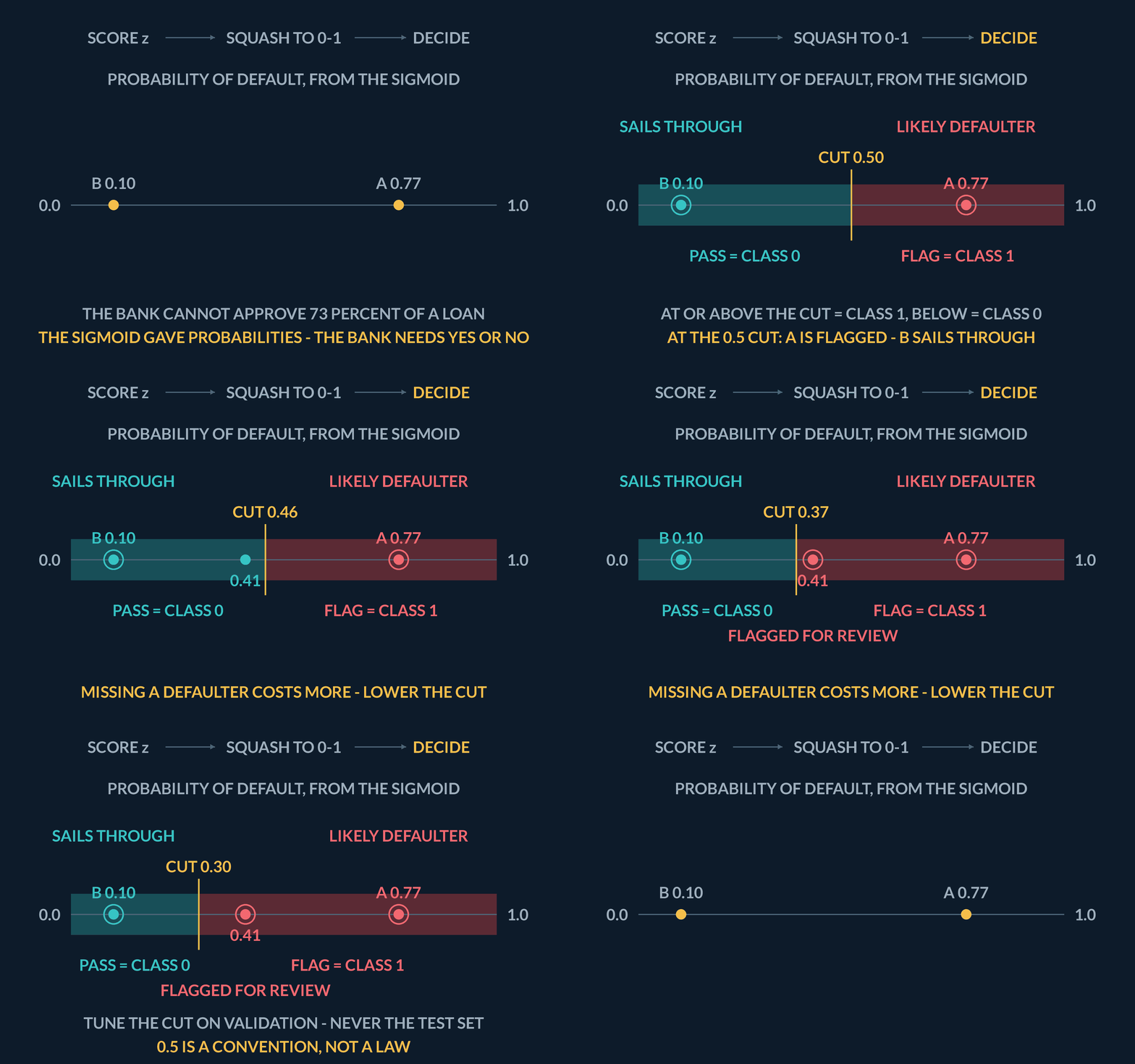
One last step turns the probability into an action. The bank cannot approve "73% of a loan" — it must decide yes or no. So we pick a threshold, a cut-off probability: at or above it we call the row class 1, below it class 0. Put the two applicants the sigmoid walk judged by hand on that 0-to-1 rail: at the common default cut of 0.5, A at 0.77 is flagged as a likely defaulter and B at 0.10 sails through. But 0.5 is a convention, not a law. If missing a defaulter costs the bank far more than annoying a safe applicant with extra checks, lower the cut — say to 0.3 — and a borderline applicant at 0.41, who passed a moment ago, now gets flagged for review. The same probability, a different decision: the threshold is a dial the bank sets deliberately, not part of the model. Tune that choice on validation data — data held aside from training — never on the final test set.
Zoom out and the whole machine is smaller than it looks: features in, the weighted sum turns them into one score z = w \cdot x + b, the sigmoid squashes z into a probability, and the threshold turns the probability into a label — repay or default. Set that beside the rent line and the family resemblance is exact: linear regression outputs a continuous number and trains on squared error; logistic regression outputs a probability and trains on log loss. Same start, different ending — and that pattern, a linear core plus a shaping function, is one you will meet again and again in machine learning.
- Build the linear scoreCompute z = w·x + b for each row — same weighted sum as linear regression.
- Map through sigmoidTurn z into P(y=1) = 1/(1+e^{-z}); compare probabilities, not raw z, when ranking rows.
- Pick a thresholdDefault 0.5 is not sacred — move it when false alarms or misses have different costs.
| Model | Output | Typical loss |
|---|---|---|
| Linear regression | Continuous ŷ | Squared error |
| Logistic regression | Probability in (0, 1) | Log loss |
Pricing three predictions about one repayer
Applicant B — scored z = -2.2 by the bank's model, a predicted default chance of about 0.10 — does in fact repay the loan. Log loss prices every prediction after the truth arrives: for a row whose true class is "repays" (class 0), the penalty is -\ln(1 - \hat{p}), where \hat{p} is the default probability the model predicted and \ln is the natural logarithm (the ln key on a calculator). Price three models that judged B: the honest one at \hat{p} = 0.10, an unsure-but-wrong one at \hat{p} = 0.60, and a shouting one at \hat{p} = 0.99. Rounded logs to use: \ln 0.90 \approx -0.105, \ln 0.40 \approx -0.916, \ln 0.01 \approx -4.605.
- Honest model: it left 1 - 0.10 = 0.90 of probability on the outcome that actually happened, so its penalty is -\ln 0.90\approx 0.105
- Unsure-but-wrong model at 0.60: probability left on the true outcome is 1 - 0.60 = 0.40, penalty -\ln 0.40\approx 0.916
- Shouting model at 0.99: it left only 1 - 0.99 = 0.01 on what happened, penalty -\ln 0.01\approx 4.605
- How much harder the confident miss is punished than the unsure one: 4.605 \div 0.916\approx 5\times
- And against the honest call at 0.10: 4.605 \div 0.105\approx 44\times
Pro tip. The 0.5 threshold appears nowhere in these penalties. Log loss reads the raw probability during training and sets the weights; the threshold is bolted on afterwards to turn probabilities into decisions. Moving the cut from 0.5 to 0.3 changes who gets flagged — it changes nothing about what the model learned.
How does changing the classification decision threshold from 0.5 to 0.2 affect a fraud detector?
- It changes the underlying logistic regression weights fitted during training
- It flags more transactions as fraud, increasing recall at the expense of catching more false alarms
- It decreases the number of predicted positive cases across the dataset
- It guarantees that precision and recall both reach 100% simultaneously
Lowering the decision threshold makes the model more aggressive at predicting the positive class (fraud), catching more actual frauds (higher recall) while incurring more false positives (lower precision).
4Lab: logistic baseline
Time to stop reading and fit one. The lab uses scikit-learn's `LogisticRegression` — a ready-made implementation of everything the previous concept described: it learns the weights w and bias b from training rows, and its predictions are sigmoid probabilities turned into class labels at the 0.5 threshold. You do not implement the sigmoid yourself; you hand the library a table of features and a column of true labels, and it does the fitting.
The first cell builds a small fake dataset with `make_classification` (fake is fine — the point is the workflow, not the data), then immediately splits it into a training set and a test set with `train_test_split`. Why split before doing anything else? Because the score you report must come from rows the model never saw during fitting — that held-out score is called hold-out accuracy, and it is your only honest estimate of how the model handles new data. Scoring on the same rows the model trained on is like grading a student on the exact questions they memorised: the number looks great and means nothing. This fit-then-score-on-held-out-rows pattern is the skeleton every later applied lesson reuses.
Two small settings in the code deserve a sentence each. `n_samples=400` keeps the dataset a few hundred rows — this lab runs inside your browser, and small data keeps every re-run instant; real production tables can wait. `random_state=0` pins the random shuffle used by the split, so the same rows land in train and test every time you press run. Without it, each run would draw a different split and a different score, and you could never tell whether a change you made helped or you just got a luckier shuffle.
The second cell paints the model's decision regions: it colours every point of the feature plane by which class the fitted model would predict there. The border between the two colours is the decision boundary — the set of points where the score z is exactly 0 and the probability is exactly 0.5. Notice it is a straight line, not an S-curve: the sigmoid bends the probability, not the boundary, because the boundary sits wherever the linear score crosses zero.
Finally, treat the printed accuracy as a baseline — the simple number your next models must beat — not a leaderboard entry. And carry one question into the next lesson: if only 1 row in 100 were a defaulter, a model that always said "repays" would score 99% accuracy while catching nobody. Would accuracy still be the right headline then? That doubt is exactly where precision and recall come in.
No diagram — the fit is drawn by the coding lab plot, not a static figure.
| Step | Why |
|---|---|
| Hold out a test fold | Score must use rows the fit never saw |
| Fit LogisticRegression | Linear score → sigmoid → class probability |
| Plot decision regions | See where the probability threshold splits the plane |
Coding lab. Logistic regression baseline runs in the app, with checks on your output.
The lab paints the decision regions of a logistic model on two features. What shape is the border between the two regions?
- An S-shaped curve, because the sigmoid is S-shaped
- A circle centred on the class means
- A jagged, blocky edge that follows the training points
- A straight line — the boundary sits where z = 0, and z is linear in the features
The sigmoid curves the probability, not the boundary. The classes divide where z = w \cdot x + b = 0, which is a line in the feature plane.
Notes
- Logistic regression still computes a linear score z = w·x + b, then maps it through a sigmoid to a probability between 0 and 1.
- Despite the name it is a classifier: the continuous output is P(class = 1), not a rent price or a count.
- A threshold (often 0.5, sometimes tuned on validation) turns the probability into a hard label.
Exam traps & shortcuts
- Keep lab datasets under 2000 rows in the browser runtime.
- Split train and test before fitting any model that sees labels.
Recap
This lesson in brief:
- Logistic regression
- Logistic regression still computes a linear score z = w·x + b, then maps it through a sigmoid to a probability between 0 and 1.
- Classifier, not regressor
- Despite the name it is a classifier: the continuous output is P(class = 1), not a rent price or a count.
- Threshold
- A threshold (often 0.5, sometimes tuned on validation) turns the probability into a hard label.
Practise Logistic Regression
Reading is free and needs no account. Practice, mocks and progress live in the app.
- 10 exam-style questions on this topic, with explanations
- A 5-question practice set that ends the chapter
- Timed mocks scored with the real marking scheme
- Readiness tracked per topic, kept on your device