Machine Learning · Machine Learning Core
Linear Regression
Predict a continuous target as a weighted sum of features — the first classical model, with an in-browser OLS lab.
After the split is locked, the first model is often a straight line: ŷ = w·x + b fitted by ordinary least squares. This lesson teaches that geometry alone, then lets you fit and plot it in the browser.
- Machine Learning
- Easy level
- 4 concepts
- 10 practice questions
1From features to a guess
Suppose you want to guess the monthly rent of a flat you have never seen. You do know a few things about it: how many bedrooms it has, and how far it is from the city centre. Facts like these — numbers you know before you know the answer — are called features. The number you are trying to guess — the rent — is called the target. Linear regression is a recipe for turning features into a guess at the target.
The recipe is deliberately simple: start from a base amount, then add or subtract a fixed amount for each feature. For the flat, that might be "start at ₹8,000, add ₹250 per bedroom, subtract ₹120 per kilometre from the centre." Written compactly this is \hat{y} = w \cdot x + b. Read every symbol: \hat{y} is pronounced "y-hat" and is the model's guess at the target — the hat marks it as an estimate, not the true rent. x stands for the features: the bedroom count and the distance. w is the list of weights, one number per feature, saying how much each feature pushes the guess up or down (₹250 per bedroom is a weight; so is −₹120 per kilometre). b is the bias, also called the intercept — the starting value the guess takes when every feature is zero. The dot in w \cdot x just means "multiply each feature by its weight, then add the results up", so the whole recipe is a weighted sum of the features plus a starting value.
| Piece | Role |
|---|---|
| Features x | Inputs known at predict time |
| Weights w, bias b | Fitted parameters |
| Squared error | Usual training loss (OLS) |
| Residual | y − ŷ; plot these before celebrating R² |
Running the recipe: two flats through the weighted sum
Use the topic's fitted rent line, \hat{y} = 8000 + 250 \cdot \text{bedrooms} - 120 \cdot \text{km_to_hub}, with the guess coming out in rupees per month. Two new flats need guesses: flat A has 1 bedroom and sits 3 km from the hub; flat B has 3 bedrooms and sits 10 km out. Run each flat through the recipe part by part — the base amount, the bedroom term, the distance term, the total — and then explain, from the terms alone, why the flat with more bedrooms ends up with the lower guess.
- Ground the bias first. A flat scoring zero on every feature — a 0-bedroom studio at the hub itself — gets 8000 + 250 \times 0 - 120 \times 0: both weighted terms vanish and only the starting value remainsRs 8,000 — the bias is the guess when the features say nothing
- Flat A's bedroom term, weight times feature: 250 \times 1+250
- Flat A's distance term: -120 \times 3−360
- Flat A's guess, base plus both terms: 8000 + 250 - 360Rs 7,890
- Flat B, same recipe: bedroom term 250 \times 3 = 750, distance term -120 \times 10 = -1200, total 8000 + 750 - 1200Rs 7,550
- Why did three bedrooms lose to one? Compare the terms. Going from flat A to flat B, bedrooms add 750 - 250 = 500 more, but distance takes 1200 - 360 = 840 more away; the net move is 500 - 840 = -340, and indeed 7890 - 340Rs 7,550 — the weighted sum lets one feature outvote another
Pro tip. Do not rank features by the size of their weights. Rs 250 per bedroom looks bigger than Rs 120 per kilometre, but bedrooms range over a few units while distance ranges over many: across flat B's 10 km, distance moved the guess by Rs 1,200 — outvoting all Rs 750 of its bedrooms. A weight is a price per unit; a feature's influence is that price times how far the feature actually varies.
In linear regression with equation y_hat = w1*x1 + b, what does the bias term b represent physically?
- The slope indicating how sharply y_hat responds to changes in x1
- The sum of squared residuals across the entire training partition
- The baseline prediction when all input features x_i evaluate to zero
- The ratio of input feature variance to target label variance
The bias (or intercept) b provides the baseline value when all feature inputs x_i are zero, shifting the line up or down independently of the slopes.
2Least squares picks the line
So where do the weights and the bias come from? Nobody types them in — the model learns them from example flats whose true rents are already known, called the training rows. Here is how the learning works. Pick any candidate line, meaning any choice of w and b. For each training flat, compare the guess \hat{y} against the true rent y; the difference is that row's error. Square each error and add them all up across the training rows. Ordinary least squares — OLS for short — is the rule that says: choose the w and b that make this total of squared errors as small as possible. Why square the errors instead of just adding them? Two reasons. Squaring stops a guess that is too high from cancelling a guess that is too low — a +4 error and a −4 error would otherwise sum to zero and look perfect. And squaring makes big misses hurt disproportionately: missing by 2 costs 2^2 = 4, four times the cost of missing by 1 — the right behaviour whenever one large mistake is worse than several tiny ones.
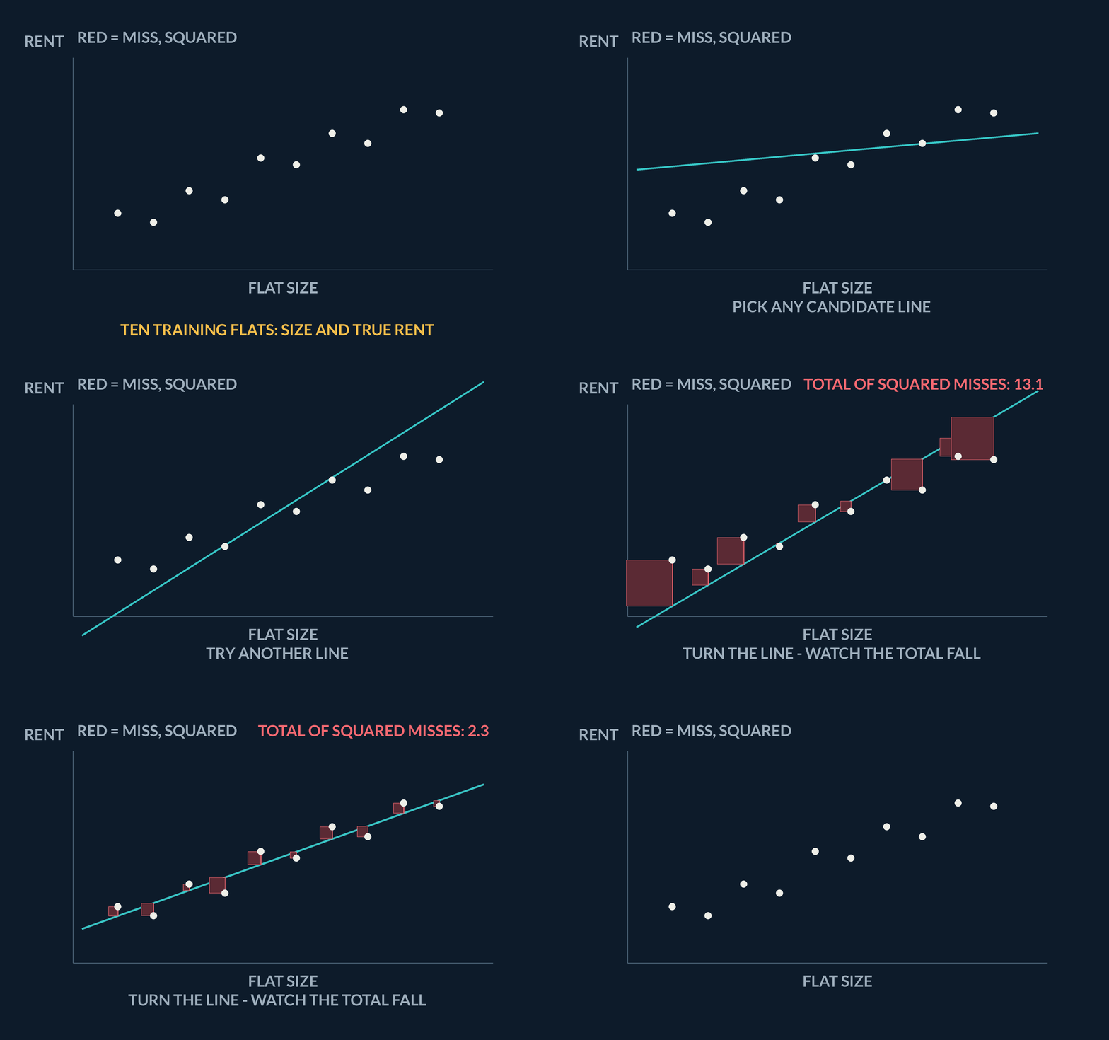
- Split firstHold out test rows before fitting — OLS must never see labels from the evaluation fold.
- Fit on trainMinimise squared error on X_train, y_train; read intercept and slopes from the fitted object.
- Score on testReport R² or RMSE on X_test only — the metric that estimates generalisation.
| Scoring step | Candidate A: the fitted line | Candidate B: always guess the average |
|---|---|---|
| Guesses for 1, 2, 3 bedrooms | ₹7,650, ₹7,900, ₹8,150 | ₹7,900 for every flat |
| Errors y - \hat{y} | +50, -50, 0 | -200, -50, +250 |
| Plain sum of errors | 0 — looks perfect | 0 — the ₹200 and ₹250 misses cancel |
| Total of squared errors | 2,500 + 2,500 + 0 = 5,000 | 40,000 + 2,500 + 62,500 = 105,000 |
| OLS verdict | Kept — 21 times smaller total | Rejected — the single ₹250 miss alone costs 62,500 |
Two candidate lines, one squared-error verdict
Three training flats sit at the same 5 km from the hub, so only bedrooms vary. True rents: 1 bedroom → ₹7,700, 2 bedrooms → ₹7,850, 3 bedrooms → ₹8,150 per month. Candidate A is the familiar line \hat{y} = 8000 + 250 \cdot \text{bedrooms} - 120 \cdot \text{km_to_hub}. Candidate B ignores bedrooms entirely and always guesses one number: the average of the three true rents. Compute each candidate's total squared error and say which line ordinary least squares keeps — and why adding the plain, unsquared errors cannot decide it.
- Candidate A's guesses. Every flat is 5 km out, so the distance term is fixed at -120 \times 5 = -600 and the line collapses to \hat{y} = 7400 + 250 \cdot \text{bedrooms}₹7,650, ₹7,900, ₹8,150
- Candidate B's one guess is the average of the three true rents, offered for every flat regardless of bedrooms: (7700 + 7850 + 8150)/3 = 23700/3₹7,900 for every flat
- Each row's error is true rent minus guess, y - \hat{y}, positive when the guess is too lowA: +50, -50, 0; B: -200, -50, +250
- Try the naive scoring first — just add the errors. A: 50 - 50 + 0; B: -200 - 50 + 250. A guess that is too high cancels a guess that is too low, so B's misses of ₹200 and ₹250 vanish from its total, and plain sums cannot choose between these linesboth totals: 0
- Now square each error before adding, as OLS does. A: 50^2 + (-50)^2 + 0^2 = 2500 + 2500 + 0; B: (-200)^2 + (-50)^2 + 250^2 = 40000 + 2500 + 62500A: 5,000; B: 105,000
- Compare the totals — 21 times smaller. Squaring is exactly what let the two totals disagree, and it punished B hardest for its single biggest miss: the ₹250 error alone contributed 250^2 = 62500, more than half of B's totalOLS keeps candidate A
Pro tip. Candidate B is not a straw man. 'Always guess the average' is the zero-weight line every fitted model must beat, and it is the exact baseline that R² measures against — an R² near 0 means your line did no better than guessing the mean.
Why does Ordinary Least Squares minimise the sum of squared errors rather than raw errors (y - y_hat)?
- Raw errors cannot be computed when predictions exceed true values
- Raw errors cancel out positive and negative misses, whereas squaring makes all penalties positive and penalises large deviations heavily
- Squaring shrinks large prediction outliers down to zero penalty
- Least squares is strictly required to run in sub-millisecond execution time
Raw errors sum to zero for any line passing through the centroid. Squaring ensures every deviation is penalised positively and grows quadratically with error size.
3Read the weights, check the residuals
Once the model is fitted, each weight has a plain-language reading. If the weight on bedrooms is 250, then adding one bedroom raises the predicted rent by 250 — provided every other feature stays exactly the same. That last clause matters. The reading is only trustworthy when the features are on sensible, comparable scales, and when no two features are near-copies of each other. Two features that always move together — say, distance in kilometres and the same distance in metres — are called collinear, and the model can split their shared effect between them in arbitrary ways, leaving each individual weight meaningless even though the predictions stay fine.
Finally, never celebrate a fit without looking at what it got wrong. For each row, the residual is y - \hat{y}: the true value minus the guess, the leftover the line could not explain. A positive residual means the model guessed too low for that row; a negative one means it guessed too high. You will also meet R^2, pronounced "R-squared": a single score between 0 and 1 that says how much of the target's variation the line accounts for, higher being better. But R^2 is one number and cannot show you where the line fails. So treat the fitted line as a baseline, not a truth: plot the residuals against the feature, and if they rise, then fall, then rise again — curving instead of scattering randomly — the data is bending and your straight line is the wrong shape, no matter how healthy the R^2 looks.
Figure. Residuals plotted against the feature. A healthy fit scatters them randomly around the zero line; here they rise, then fall, then rise again — the data is bending, and a straight line is the wrong shape no matter how healthy the R-squared looks.
| Number | Reading in rupees |
|---|---|
| Bias b = 8000 | Where the guess starts: ₹8,000 for a flat where every feature is zero |
| Weight 250 on bedrooms | One more bedroom raises the predicted rent by ₹250 — trustworthy only while every other feature stays exactly the same |
| Weight -120 on km_to_hub | Each kilometre farther from the centre lowers the predicted rent by ₹120, other features held fixed |
| Residual y - \hat{y} | Positive: the model guessed too low for that flat; negative: too high — and residuals curving with the feature mean the straight line is the wrong shape |
Reading the weights back out, then the leftovers
The fitted line is still \hat{y} = 8000 + 250 \cdot \text{bedrooms} - 120 \cdot \text{km_to_hub}, guesses in rupees per month. Three flats now carry both a guess and a known true rent: flat P (1 bedroom, 2 km from the hub) rents at Rs 8,100; flat Q (2 bedrooms, 2 km) at Rs 8,180; flat R (2 bedrooms, 8 km) at Rs 7,690. First recover each weight's plain-language reading directly from the predictions, using pairs of flats that differ in exactly one feature; then compute each flat's residual y - \hat{y} and say what its sign means.
- Predictions first. Flat P: 8000 + 250 \times 1 - 120 \times 2 = 8000 + 250 - 240Rs 8,010
- Flat Q: 8000 + 250 \times 2 - 120 \times 2 = 8000 + 500 - 240Rs 8,260
- Flat R: 8000 + 250 \times 2 - 120 \times 8 = 8000 + 500 - 960Rs 7,540
- Read the bedroom weight from a clean pair: flats P and Q sit at the same 2 km and differ by exactly one bedroom, so the prediction gap is 8260 - 8010Rs 250 — the bedroom weight, recovered exactly, because the other feature stayed fixed
- Read the distance weight the same way: flats Q and R share 2 bedrooms and differ by 6 km, so the gap is 7540 - 8260 = -720, and per kilometre -720 \div 6−Rs 120 per km
- Now the residuals, true rent minus guess. Flat P: 8100 - 8010; flat Q: 8180 - 8260; flat R: 7690 - 7540+90, −80, +150
- Read the signs: the line guessed Rs 90 too low for P and Rs 150 too low for R (positive residuals), Rs 80 too high for Q (negative). Small, mixed-sign leftovers sitting on both sides of zero are what a healthy fit leaves behindno one-sided pattern — nothing here accuses the line's shape
Pro tip. The 'one more bedroom adds Rs 250' reading worked only because flats P and Q agreed on distance. In real data no such clean pair may exist, and two near-copy features — distance in kilometres beside the same distance in metres — let the fit split one effect between them arbitrarily, wrecking both readings while every prediction stays fine. Trust a weight's story only after checking the features are not telling it twice.
A fitted line reports a healthy R², but the residuals rise, then fall, then rise again as x grows. What should you conclude?
- The fit is fine — R² already accounts for residual shape
- The residuals need to be squared before judging them
- More training rows will straighten the residual pattern
- The line is the wrong shape for this data even though R² looks fine
Residuals that curve with x mean the model class missed structure. R² is a single number and cannot show where the line bends away from the cloud.
4Lab: fit a line
Time to actually fit a line, right here in the browser. The lab builds a small practice dataset of 200 rows with one feature (a single input column) and a target that follows a straight line plus random noise — small random nudges added on purpose, so the points scatter around the line the way real measurements do instead of sitting on it perfectly. One feature is enough for the whole fit to be drawable as a picture.
Cell 1 does three things, in order. First, train_test_split locks a quarter of the rows away as the test fold — rows the model is never allowed to look at while learning, kept aside purely to check the finished model; the remaining three quarters become the training fold. Second, model.fit(X_train, y_train) runs ordinary least squares from the previous concept on the training rows: it searches for the weight and bias that make the total squared error smallest. The printed "coef" is that fitted weight w, the slope of the line, and "intercept" is the fitted bias b, where the line sits when the feature is zero. Third, model.score(X_test, y_test) prints R^2 measured on the held-out test rows — the score that estimates how the model would do on data it has never seen, which is the only score that matters.
Cell 2 draws the result. It works because both cells run inside one shared Python session, called the kernel: the model, X_train, and y_train created in Cell 1 are still alive in memory, so Cell 2 simply scatters the training points and lays the fitted line through them — no refitting happens. Want a different title or colour? Edit Cell 2 and re-run only that cell; the fit from Cell 1 is untouched.
One honesty rule holds the whole exercise together: the printed score is trustworthy only because the fit never saw X_test before score was called. If the test rows had leaked into the fitting step, the score would flatter the model and tell you nothing about how it handles new data.
And the plot itself is the real diagnostic. Look at how the training cloud sits around the line: points scattered evenly above and below it is what a good fit looks like. But if the cloud visibly curves while the line stays straight, the model class is wrong for this data — a straight line simply cannot bend — and that mismatch can hide behind a respectable-looking R^2. The picture shows what the single printed number cannot.
No diagram — the fit is drawn by the coding lab plot, not a static figure.
| Step | Why |
|---|---|
| Hold out a test fold | Score must use rows the fit never saw |
| Fit LinearRegression | OLS picks w and b on the training fold |
| Plot the line on train | Residuals you can see beat a lone R² |
Coding lab. Fit a straight line runs in the app, with checks on your output.
In the lab, why draw the fitted line through the training cloud instead of trusting the printed R² alone?
- A curved cloud under a straight line can still print a respectable R² — the plot shows the mismatch
- The plot recalculates the score more precisely
- R² is only defined for two-feature tables
- Plotting refits the model on the test rows
The plot is the residual check you can see: if the cloud bends and the line does not, the model class is wrong regardless of the printed score.
Notes
- Linear regression predicts a continuous target as a weighted sum of features plus a bias: ŷ = w·x + b.
- Ordinary least squares picks the weights that minimise squared error on the training rows.
- Read the fit as a baseline: if residuals curve with x, the line is the wrong shape even when R² looks fine.
Exam traps & shortcuts
- Keep lab datasets under 2000 rows in the browser runtime.
- Split train and test before fitting any model that sees labels.
Recap
This lesson in brief:
- Linear regression
- Linear regression predicts a continuous target as a weighted sum of features plus a bias: ŷ = w·x + b.
- Ordinary least squares
- Ordinary least squares picks the weights that minimise squared error on the training rows — the default loss when "miss by 2" should hurt four times as much as "miss by 1".
Practise Linear Regression
Reading is free and needs no account. Practice, mocks and progress live in the app.
- 10 exam-style questions on this topic, with explanations
- A 5-question practice set that ends the chapter
- Timed mocks scored with the real marking scheme
- Readiness tracked per topic, kept on your device