Machine Learning · Machine Learning Core
Regularisation
Why huge weights chase noise, and how an L2 (ridge) penalty charges weight size so a coincidence no longer wins the training-loss contest.
A spam filter can buy a slightly smaller training loss — one number for how wrong it is on the two hundred labelled emails it studied — by hanging a huge weight on a coincidence word. Regularisation adds a second charge to that bill: a penalty on the size of the weights. This lesson walks one mental model, slowly: what a weight is, why an ordinary fit (the fit that only looks at training loss) keeps the huge one, how an L2 (ridge) penalty prices that size, and how scikit-learn's Ridge tool turns the same price with a knob called alpha.
- Machine Learning
- Medium level
- 6 concepts
- 4 practice questions
1Huge weights chase noise
Picture a student preparing for an exam by memorising last year's paper word for word. On those exact 200 questions they score 100%. On a fresh paper they collapse, because they never learned the subject — they learned the quirks of one specific question set. A model can fail in exactly the same way: it can score brilliantly on the rows it was trained on and badly on new rows. That failure has a name — overfitting.
Training loss is one number that says how wrong the model is on the rows it studied — smaller is better. Overfitting is what happens when the fit is allowed to buy a slightly smaller training loss with a story that will not repeat on fresh rows.
No diagram — the memorising-student table carries the analogy.
| Memorising student | Overfitting model | |
|---|---|---|
| What gets learned | Last year's paper, word for word | A huge weight on a coincidence that will not repeat |
| On seen material | 100% on those exact 200 questions | Brilliant score on the training rows |
| On fresh material | Collapses on a fresh paper | Fails on new rows the fit never studied |
| Why it happens | Learned the quirks of one question set, not the subject | The huge weight bought a slightly better training loss |
When an unregularised linear model overfits noisy colinear features, what commonly happens to its learned weights?
- All weights collapse to exactly zero, producing a constant horizontal line
- The bias term becomes strictly equal to the learning rate parameter
- The weights explode into massive positive and negative values that cancel out on training rows but fail on new data
- The model automatically converts itself into an ensemble of decision trees
Without constraints, colinear features allow weights to grow excessively large in opposite directions to fit small idiosyncrasies in the training sample.
2Where overfitting lives: one huge weight
The running example for this whole lesson is a spam filter: a small program that reads an incoming email and answers one question — spam, or not spam. You build it by showing it 200 old emails, each already labelled spam or safe, and letting it learn from them. That learning step is called training. The filter keeps one learned number per clue word — per word, like how often FREE appears. That number is a weight, written w. A weight of +2 on FREE means that word pushes the score firmly toward spam. A weight near 0 means the filter barely listens to that word.
Suppose the word "meeting" happened, by pure coincidence, to appear in three spam emails in the training pile. An ordinary fit — the fit that only looks at training loss — will happily give "meeting" a huge weight, say w = +7, because that buys a slightly better training-loss number on those 200 emails. On next week's inbox, where "meeting" means a meeting, that huge weight is a liability. The training-loss win was a quirk, not a subject.
Figure. The spam filter keeps one learned weight w per clue: +2 on FREE pushes firmly toward spam, a weight near zero is barely heard. An ordinary fit — the fit that only looks at training loss — hands meeting a huge +7 because that word happened to appear in three training spams. The slightly better training-loss number is a coincidence, and the huge weight becomes a liability on next week's inbox.
| Word | Weight w | What it means |
|---|---|---|
| FREE | +2 | Listens firmly — that word pushes toward spam |
| typical word | near 0 | Barely heard |
| meeting (3 coincidences) | +7 | Huge — bought a slightly better training loss on a quirk |
A model assigns a weight of +500 to an unscaled feature that fluctuates by +/- 2. What is the consequence?
- The model becomes entirely insensitive to variations in that feature
- The feature's coefficient is automatically pruned during inference
- The training loss increases exponentially on every training iteration
- Minor noise in that feature creates huge wild swings of +/- 1000 in the final prediction
A huge coefficient acts as an amplifier: tiny noise in the input creates massive swings in the output, leading to erratic test predictions.
3An ordinary fit keeps the huge weight
Who chooses the weights? Nobody types them in. Training does. Training tries out weight settings, scores each one, and keeps the setting with the best score. That is the entire game: not a person picking by taste, and not a vote from next week's inbox — a search for the cheapest score on the rows the model is allowed to study.
An ordinary fit is the fit whose bill is training loss alone. Two candidate settings for the spam filter: setting A hangs w = +7 on meeting and scores training loss 0.10 (its "how wrong on the 200 training emails" number). Setting B hangs only w = +0.5 on meeting and scores training loss 0.30. Smaller training loss wins, so 0.10 beats 0.30 and training keeps the monster. Next week's inbox, where that monster embarrasses us, is not on the scoreboard.
Figure. An ordinary fit scores only training loss. Setting A (meeting weight +7) has training loss 0.10; setting B (meeting weight +0.5) has training loss 0.30. Smaller wins, so the ordinary fit keeps the huge weight. Next week's inbox is not on this scoreboard.
| Setting | Meeting weight w | Training loss | Ordinary-fit winner? |
|---|---|---|---|
| A | +7.0 | 0.10 | Yes — 0.10 is smaller |
| B | +0.5 | 0.30 | No — 0.30 is worse on the training emails |
Why does standard OLS linear regression allow weights to become excessively large during training?
- OLS contains an internal bug that doubles weight values on every iteration
- Matrix inversion requires all singular values to be strictly negative
- OLS objective cares solely about minimising training squared error with zero penalty on weight magnitudes
- OLS automatically maximises coefficient variance across features
OLS minimizes squared error alone. If inflating weights reduces training error by even a tiny fraction, OLS will do so without constraint.
4Charge the size of the weights
Regularisation is the fix, and the idea is simple: charge the model for the size of its weights. The extra charge is called a penalty — a second number, added to training loss, that grows as the weights grow. A huge weight on "meeting" is no longer free. Training still tries settings and keeps the cheapest one — that part never changes — but cheapest now means cheapest on the whole bill, loss and penalty together. The fit keeps a large weight only if that weight earns its cost by genuinely improving predictions. Three coincidental emails no longer qualify.
This lesson uses one standard size-bill, called L2 or ridge: add up the squares of the weights. If the two headline weights are w_1 on FREE and w_2 on meeting, the size-bill is w_1^2 + w_2^2. Squaring punishes a 7 much harder than a 0.5 — 7^2 = 49, while 0.5^2 = 0.25. The total bill the fit now minimises is training loss plus \lambda times that size-bill. \lambda (lambda) is a price you choose, not a number the model learns: it says how many points of training loss you are willing to spend per unit of size-bill.
Figure. The same two fits, priced at two λ settings. Numbers on the grid are the total bills: at weak λ=0.001 Fit A wins 0.153 to 0.304; at strong λ=0.01 Fit B wins 0.3425 to 0.63.
| Symbol | What it is |
|---|---|
| Training loss | How wrong this fit is on the 200 training emails — smaller is better |
| w | A weight: one learned number per clue word |
| w_1 | The weight on FREE — how hard the filter listens to FREE |
| w_2 | The weight on meeting — how hard it listens to the coincidence word |
| Penalty / size-bill w_1^2 + w_2^2 | L2 (ridge): square each weight, then add |
| \lambda (lambda) | The price you set on each unit of that size-bill |
| Total bill | Training loss + \lambda × size-bill — the number the fit actually minimises |
What is the core modification that regularised regression makes to the standard loss function?
- It multiplies the training loss by the total number of input features
- It adds a penalty term proportional to weight magnitude, forcing the fit to balance accuracy against complexity
- It discards the training labels and runs unsupervised dimensionality reduction
- It replaces the gradient descent optimizer with random sampling
Regularization alters the objective to Loss + Penalty(w), charging a cost for large weights so the model avoids chasing noise.
5The 0.20 versus 48.75 tug-of-war
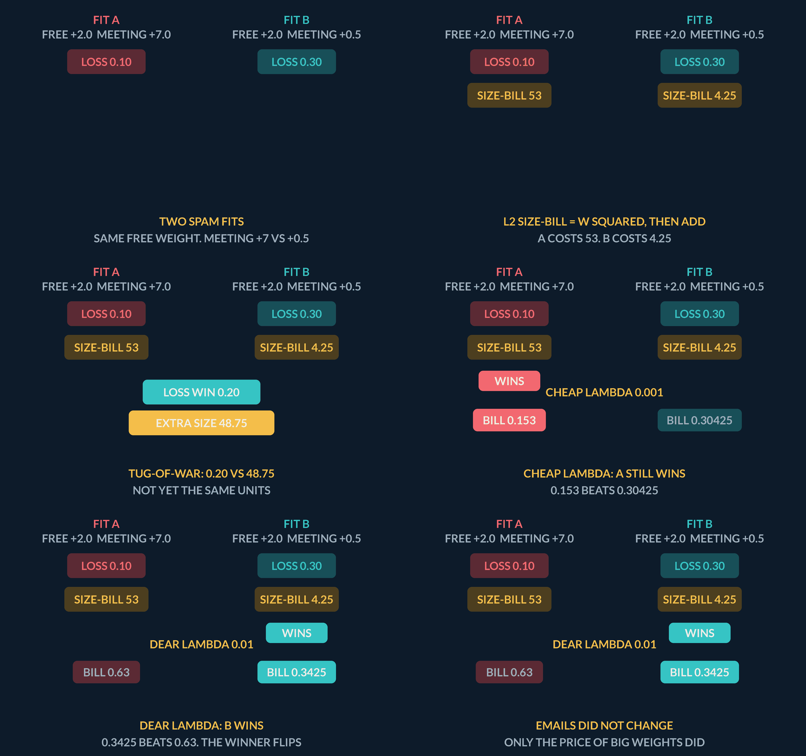
Keep the same two spam-filter settings. Both listen to FREE at w_1 = +2.0. Setting A listens to meeting at w_2 = +7.0 and has training loss 0.10. Setting B listens to meeting at w_2 = +0.5 and has training loss 0.30. The L2 size-bill is w_1^2 + w_2^2. For A that is 2.0^2 + 7.0^2 = 4 + 49 = 53. For B that is 2.0^2 + 0.5^2 = 4 + 0.25 = 4.25. A pays 53 - 4.25 = 48.75 extra size-bill for the privilege of the huge meeting weight. What does A buy with that extra size? A training-loss number that is 0.30 - 0.10 = 0.20 smaller. So the tug-of-war is 0.20 of training-loss win versus 48.75 of extra size-bill.
Those two numbers are not yet in the same units. \lambda is the exchange rate: each unit of size-bill costs \lambda points of training loss. At a cheap price \lambda = 0.001, A's extra 48.75 of size costs only 0.001 \times 48.75 = 0.04875 — less than the 0.20 it saves, so A still wins. At a dear price \lambda = 0.01, the same extra size costs 0.01 \times 48.75 = 0.4875 — more than the 0.20 it saves, so B wins. The emails did not change. Only the price of big weights did.
Name every number, then add the bill
Two candidate spam fits. Fit A leans on the coincidence: weight +2.0 on FREE (listens firmly to FREE), weight +7.0 on meeting (listens hard to a word that appeared in three training spams), training loss 0.10 (its "how wrong on the 200 training emails" number). Fit B ignores the coincidence: the same +2.0 on FREE, only +0.5 on meeting, training loss 0.30 — worse on the training emails because it refuses the quirk. The L2 size-bill is w_1^2 + w_2^2. The total bill is training loss plus \lambda times that size-bill. Compute each fit's size-bill, the 0.20 versus 48.75 tug-of-war, then the total bill at a cheap price \lambda = 0.001 and a dear price \lambda = 0.01. Which fit wins each time?
- Fit A's size-bill: square each weight, then add. 2.0^2 + 7.0^2 = 4 + 4953
- Fit B's size-bill: 2.0^2 + 0.5^2 = 4 + 0.254.25
- A's extra size-bill versus B: 53 - 4.2548.75
- A's training-loss win versus B: 0.30 - 0.100.20
- Cheap \lambda = 0.001 means each unit of size-bill costs 0.001 of training-loss points. Fit A total: 0.10 + 0.001 \times 530.153
- Fit B at the same cheap price: 0.30 + 0.001 \times 4.250.30425
- Winner at the cheap price (smaller total bill)Fit A — 0.153 beats 0.30425
- Dear \lambda = 0.01: each unit of size-bill now costs ten times as much. Fit A: 0.10 + 0.01 \times 530.63
- Fit B at the dear price: 0.30 + 0.01 \times 4.250.3425
- Winner at the dear priceFit B — 0.3425 beats 0.63; the ordering flips
- Same tug-of-war in one line: at \lambda = 0.01, A's extra size costs 0.01 \times 48.75 = 0.4875, which is larger than the 0.20 of training loss A buys, so the huge meeting weight no longer earns its keep0.4875 > 0.20 — B wins
Pro tip. Neither fit changed and neither did the emails — only the price of big weights did. At the dear setting, fit A's meeting weight alone costs 0.01 \times 7^2 = 0.49 of penalty, more than the 0.20 of training loss it buys (0.30 - 0.10), so it no longer earns its keep.
In Ridge regression MSE + alpha * sum(w_j^2), what happens if you set alpha to an extremely large value?
- The penalty dominates, shrinking all feature weights near zero and causing underfitting
- The model overfits the training set and achieves zero training loss
- The weights diverge to positive infinity due to gradient explosion
- The algorithm stops after a single gradient descent step
A massive alpha prioritizes shrinking weights above fitting the data, collapsing coefficients toward zero and producing a high-bias underfit model.
6The same price in scikit-learn
A Python library is a bundle of ready-made tools someone else already wrote, so you do not have to type the maths by hand. scikit-learn is one such library for machine learning. The short name you type in Python is sklearn. The line `import sklearn` loads the library. The everyday line is `from sklearn.linear_model import Ridge` — that reaches into the linear-model drawer inside the library and pulls out one tool, Ridge. Ridge is the name scikit-learn gives the L2 (ridge) fit you just priced by hand: it still tries to make training loss small, and it still adds \lambda times the sum of squared weights.
Two verbs do the work. `fit` means study the training rows and pick the weights. `predict` means use those learned weights on new rows. The penalty knob on Ridge is called `alpha`. It is the same idea as lambda: a bigger `alpha` is a dearer price on big weights. The lab below fits the same four-row table twice — once at `alpha=0.01` (cheap) and once at `alpha=10` (dear) — and prints the two weights. Expect the dear setting to shrink both numbers. Same L2 bill — one line of code. You do not need the rest of the library today.
Figure. scikit-learn is a Python library imported as sklearn. Ridge is the L2 tool inside it. alpha is the same price as lambda. fit studies the training rows and picks weights; predict uses those weights on new rows. At a cheap alpha of 0.01 the two weights stay near 2.00 and 1.98; at a dear alpha of 10 they shrink to about 0.67 and 0.18.
| Setting | Weights (FREE, meeting) | What it means |
|---|---|---|
| `alpha=0.01` (cheap λ) | about 2.00, 1.98 | Almost the ordinary 2 and 2 — a cheap price barely moves the weights |
| `alpha=10` (dear λ) | about 0.67, 0.18 | Both weights shrink; the meeting-like column shrinks more |
| `predict([1, 1])` at alpha 10 | about 0.85 | fit already picked the weights; predict only uses them on a new row |
Ridge in four lines
import sklearn
from sklearn.linear_model import Ridge
model = Ridge(alpha=0.01)  # alpha is λ
model.fit(X, y)            # study rows, pick weights
guesses = model.predict(X_new)
Coding lab. Watch alpha shrink the weights runs in the app, with checks on your output.
In scikit-learn's Ridge regressor, what does increasing the alpha parameter do?
- It raises the learning rate for stochastic gradient descent updates
- It strengthens the L2 penalty, pulling feature coefficients closer to zero to reduce variance
- It increases the maximum tree depth allowed during training
- It switches the loss function from mean squared error to absolute error
In Ridge(alpha=...), larger alpha increases the L2 penalty on sum(w^2), shrinking coefficients toward zero.
Notes
- Overfitting shows up as huge weights that buy a slightly better training loss on quirks that will not repeat.
- Regularisation adds a second charge — a penalty on weight size — to the training-loss bill.
- L2 (ridge) charges the sum of squared weights. A dearer price \lambda can flip which fit wins.
Exam traps & shortcuts
- Keep lab datasets under 2000 rows in the browser runtime.
- Split train and test before fitting any model that sees labels.
- Tune regularisation strength on validation, never by peeking at the final test fold.
Recap
This lesson in brief:
- The problem
- A huge weight can buy a slightly better training loss on a quirk that will not repeat — overfitting.
- Ordinary fit
- An ordinary fit scores training loss only, so 0.10 beats 0.30 and the monster weight wins.
- The fix
- Add a second charge to the bill: a penalty on the size of the weights.
- L2 / ridge
- The size-bill is the sum of squared weights. A dearer \lambda can flip which fit wins — 0.20 of loss versus 48.75 of extra size, priced by \lambda.
- scikit-learn
- Ridge is the L2 tool; `alpha` is \lambda; `fit` studies rows and `predict` uses the learned weights.
Practise Regularisation
Reading is free and needs no account. Practice, mocks and progress live in the app.
- 4 exam-style questions on this topic, with explanations
- A 4-question practice set that ends the chapter
- Timed mocks scored with the real marking scheme
- Readiness tracked per topic, kept on your device