Machine Learning · Machine Learning Core
L1, L2 and the C Dial
Pick the regularisation strength — lambda, alpha, or sklearn's flipped C — by scoring a few values on a held-out validation pile. L2 tames weights; L1 can delete.
Regularisation charges a model for the size of its weights. How hard that charge pushes is a knob you set — textbooks write it \lambda (lambda); scikit-learn's Ridge tool calls the same knob alpha; some other tools write C, which is one divided by the strength. This lesson shows they are the same kind of knob, then walks the honest way to pick a value: try a few, score each on a held-out validation pile the fit never studied, and keep the winner. It also names the two size-bills (L2 tames; L1 can delete) and lets you watch the shrink in the browser.
- Machine Learning
- Medium level
- 6 concepts
- 6 practice questions
1The knob is a price you set — lambda or alpha
Regularisation charges a model for the size of its weights — the learned numbers it hangs on each clue. How hard that charge pushes is a dial you set by hand, not a number the model learns. Textbooks write the dial as \lambda (the Greek letter lambda). A bigger lambda means a stronger charge and therefore smaller weights. scikit-learn is a Python library of ready-made tools; the short name you type is sklearn. Its Ridge tool — the ridge / L2 fit — names the same dial `alpha`. Lambda and alpha are the same kind of knob: bigger means squeeze harder.
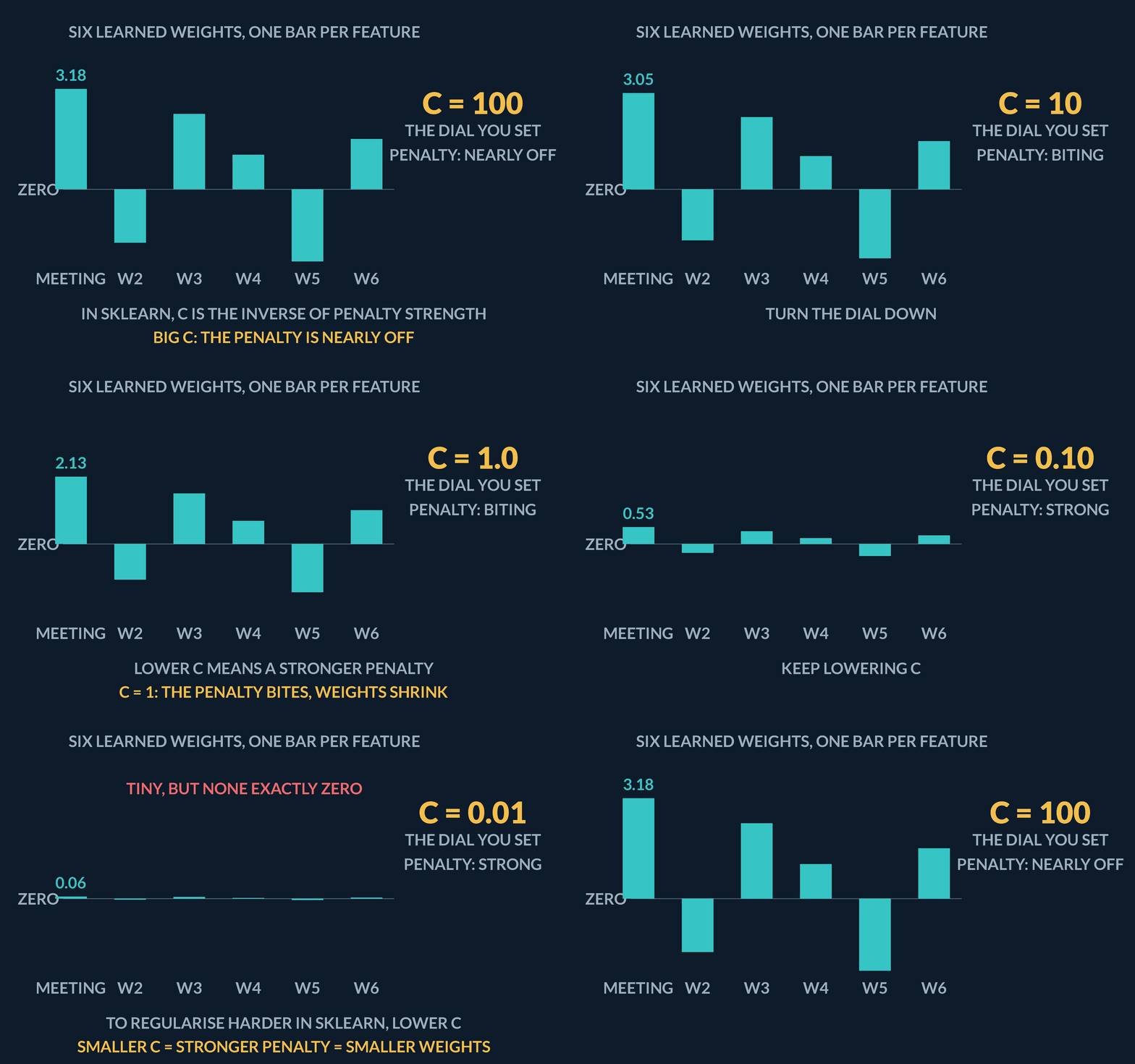
Some other tools flip the dial and call it C, defined as one divided by the strength. sklearn's LogisticRegression uses C. So a smaller C means a stronger charge — the opposite direction of lambda and alpha. To regularise harder in LogisticRegression you lower C. Raising C toward 100 or 1000 nearly switches the charge off. Meet alpha first; treat C as the same knob written upside down.
- Spot overfitTrain accuracy high and test accuracy low — coefficients may be chasing noise.
- Choose L1 or L2L2 shrinks all weights; L1 can zero some and drop features entirely.
- Tune C on validationSmaller C means stronger penalty — pick C by validation score, never by peeking at test.
| Goal | Textbook dial \lambda | sklearn dial C |
|---|---|---|
| What the number means | The penalty strength itself | The inverse of the strength |
| Regularise harder | Raise \lambda | Lower C |
| Nearly switch it off | \lambda near zero | Raise C toward 100 or 1000 |
Three names, one knob
A rent-guessing fit uses Ridge with \alpha = 10 (sklearn writes this `alpha=10`). A classmate writes the same strength as \lambda = 10. A spam-filter fit uses LogisticRegression with C = 0.1. C is defined as one divided by the strength. Which settings squeeze equally hard?
- Ridge \alpha = 10 is the same strength as \lambda = 10same knob, same number
- C is 1 divided by the strength, so C = 0.1 means strength 1 \div 0.110
- C = 0.1 and \alpha = 10 / \lambda = 10the same squeeze
Pro tip. The number ten is not a universal best setting — it is just the value that makes these three spellings match. The next concepts show how you pick a value: try a few, score each on a held-out pile.
To regularise a LogisticRegression more strongly, a classmate raises C from 1.0 to 100. What actually happened?
- The penalty got stronger, as intended
- Nothing — C only changes the number of iterations
- The model switched from L2 to L1 penalty
- The penalty got weaker — in sklearn, C is inverse strength, so a bigger C means less regularisation
Smaller C means a stronger penalty. Raising C to 100 nearly turns regularisation off; to shrink coefficients harder, lower C instead.
2Score the knob on a held-out pile
You cannot pick the knob by how well the fit does on the rows it studied. Those rows already taught the weights; a tiny lambda will look brilliant there because it was allowed to memorise quirks. The honest score uses a held-out pile: rows you cut aside before any fit starts, that the fit is never allowed to study. That pile is called the validation set. Its only job is to compare the settings you chose by hand — here, which lambda or alpha to keep.
Picture a rent office with 200 already-rented flats. Cut once, up front: 140 flats to study (the training pile), 40 flats the fit must never see while you try knob values (the validation pile), and 20 flats locked for the very end (the test pile). No flat sits in two piles. Do not pick lambda by peeking at the test pile; that headline number would then be a cheat. This lesson uses the validation pile to choose, and leaves the test pile shut.
Figure. One cut of 200 rented flats: 140 to study (train), 40 to score each knob value (validation), 20 locked until the knob is already chosen (test). Each flat lands in exactly one pile.
| Pile | How many flats | Job |
|---|---|---|
| Training | 140 | The fit studies these — it may set weights from them |
| Validation | 40 | Score each knob value; the fit never studies these |
| Test | 20 | Opened once, after the knob is chosen — never for the choice |
Why must regularisation strength alpha (or C) be chosen using validation data rather than training loss?
- Validation sets are required to calculate the L2 norm of the weights
- Scikit-learn raises an error if regularisation parameters are evaluated on train sets
- Training loss is always lowest with zero regularisation, so training data will always prefer the most overfit model
- Regularised models cannot compute gradients on training observations
On training data, unconstrained models always have the lowest loss. Only a held-out validation set reveals when regularisation prevents overfitting.
3Try a few values, keep the winner
The recipe is short. Try a few knob values. For each value, fit on the training flats only. Score that fit on the validation flats using one number: the average miss. A miss on one flat is the absolute difference |\text{actual rent} - \text{guessed rent}| — drop the sign, keep the size. Average miss means add the misses and divide by how many held-out flats you scored. Keep the knob value whose average miss is smallest.
scikit-learn can run that sweep for you. `Ridge` is the tool that fits a rent line and charges for weight size; you pass it one `alpha`. `RidgeCV` is the same tool with a built-in contest: you hand it a list of alphas, it tries each one on held-out rows, and it keeps the winner. You still have to understand the contest — the class is not magic, it is the recipe above typed once.
Figure. Average miss on three held-out flats at three alphas. The middle bar is shortest: alpha 1 wins because Rs 1,000 is smaller than Rs 3,000 and Rs 2,000. Shorter is better.
- Try a fewPick a short list of alphas — say 0.01 (gentle), 1 (medium), 100 (harsh).
- Score eachFit on training flats only. Average the absolute misses on the validation flats.
- Keep the winnerThe alpha with the smallest validation average miss is the one you keep.
One alpha, or a contest of alphas
from sklearn.linear_model import Ridge, RidgeCV

# Ridge: you already chose one alpha.
model = Ridge(alpha=1)

# RidgeCV: try the list, keep the winner.
chooser = RidgeCV(alphas=[0.01, 1, 100])
Three held-out flats, three alphas
A rent office sets three already-rented flats aside as a tiny validation pile (a real office would use more; three lets every miss be written out). Actual monthly rents: Rs 12,000, Rs 18,000, and Rs 15,000. A miss on one flat is |\text{actual} - \text{guess}|. Average miss is the three misses added, then divided by 3. Three Ridge fits, trained on other flats, guessed these rents. Find each average miss and keep the winning alpha.
- Gentle \alpha = 0.01 guesses Rs 15,000, 15,000, 18,000. Misses: |15000-12000|, |15000-18000|, |18000-15000|Rs 3000, 3000, 3000
- Average miss at \alpha = 0.01: (3000+3000+3000) \div 3Rs 3000
- Medium \alpha = 1 guesses Rs 13,000, 17,000, 16,000. Misses: |13000-12000|, |17000-18000|, |16000-15000|Rs 1000, 1000, 1000
- Average miss at \alpha = 1: (1000+1000+1000) \div 3Rs 1000
- Harsh \alpha = 100 guesses Rs 15,000, 15,000, 15,000. Misses: |15000-12000|, |15000-18000|, |15000-15000|Rs 3000, 3000, 0
- Average miss at \alpha = 100: (3000+3000+0) \div 3Rs 2000
- Compare Rs 3000, Rs 1000, Rs 2000. Smallest average miss wins\alpha = 1
Pro tip. The gentle setting chased noise and missed by Rs 3,000 a flat. The harsh setting squeezed too hard and missed by Rs 2,000. The middle setting won at Rs 1,000 — not because 1 is a magic constant, but because it scored best on flats the fit never studied. `RidgeCV(alphas=[0.01, 1, 100])` runs this same contest and keeps 1.
When searching for an optimal regularisation parameter alpha, why are candidate values typically spaced on a log scale (e.g. 0.01, 0.1, 1, 10)?
- Because regularisation effects span multiple orders of magnitude before noticeable changes occur
- Because linear spacing violates the convexity requirement of least squares
- Because log scales ensure that every candidate value achieves identical validation accuracy
- Because scikit-learn only accepts powers of ten as valid hyperparameter arguments
Hyperparameter impact spans orders of magnitude. Testing across a logarithmic grid (0.01, 0.1, 1, 10, 100) efficiently discovers the right scale.
4Two ways to charge size: L2 and L1
There are two standard ways to charge a model for the size of its weights — the learned numbers it hangs on each clue. L2, nicknamed ridge, adds up the squares. L1, nicknamed lasso, adds up the absolute values instead: |w_1| + |w_2| + \cdots. Absolute value means "drop the sign, keep the size": |-3| = 3, |0.5| = 0.5.
That small change has a striking consequence. L2 shrinks every weight toward zero but almost never lands one exactly on zero — every feature stays in, just tamed. L1 can push some weights to exactly zero. A feature whose weight is exactly zero contributes nothing: it has been deleted from the model. So L1 doubles as automatic feature selection.
No diagram here — the table names the two size-bills; the diamond figure follows.
| Penalty | Size-bill | Effect on weights |
|---|---|---|
| L2 (ridge) | Sum of squares w_1^2 + w_2^2 + \cdots | Shrinks all weights; rarely exact zeros |
| L1 (lasso) | Sum of sizes |w_1| + |w_2| + \cdots | Can zero some weights (sparse model) |
The last 0.1 of a weight, priced by L1 and L2
Take the spam filter's tamed pair of weights: +2.0 on FREE and +0.5 on the coincidence word "meeting". Price the pair under both penalties — L1 charges the sum of absolute values |w_1| + |w_2|, L2 charges the sum of squares w_1^2 + w_2^2 — then shrink the meeting weight toward zero in steps of 0.1 and track how much each penalty pays back per step. The payback schedule is the diamond-versus-rounded-budget picture in raw numbers.
- Both charges on (2.0, 0.5): L1 gives 2.0 + 0.5 = 2.5; L2 gives 2.0^2 + 0.5^2 = 4 + 0.25L1: 2.5, L2: 4.25
- Shrink meeting one step, 0.5 \to 0.4: L1 falls to 2.4, saving 0.1; L2 falls to 4 + 0.16 = 4.16, saving 0.09savings — L1: 0.1, L2: 0.09
- Keep stepping, 0.4 \to 0.3 \to 0.2 \to 0.1 \to 0: L1 saves exactly 0.1 at every step; L2's per-step savings fade: 0.07, 0.05, 0.03, then 0.01L1 flat, L2 fading
- The final step 0.1 \to 0 — actually deleting the feature: L1 still rewards it with the full 0.1; L2 rewards it with 0.1^2 - 0 = 0.01, a tenth as much0.1 vs 0.01
- Where L2's pressure went instead: shrinking the big FREE weight 2.0 \to 1.9 saves L2 4 - 3.61 = 0.39 — thirty-nine times its reward for zeroing the small weight's last step0.39
Pro tip. This is the diamond's corner in arithmetic. L1's flat per-step reward keeps paying for the final push to exactly zero, so the fit takes the corner and the feature dies; L2's quadratic charge has almost nothing left to offer near zero, so ridge parks small weights at small-but-nonzero values and spends its pressure taming the giants instead. A stronger L2 penalty shrinks harder everywhere — it still does not make that last 0.01 worth more than the prediction accuracy the weight buys.
What is the primary functional difference in learned weights between L1 (Lasso) and L2 (Ridge) penalties?
- L2 sets weights to zero while L1 leaves all weights completely unconstrained
- L1 applies only to classification models while L2 applies only to regression models
- L1 drives non-essential weights to exactly zero for feature selection, whereas L2 shrinks all weights smoothly
- L2 guarantees 100% training accuracy while L1 minimizes execution runtime
L1 regularization produces sparse models by driving coefficients of redundant features to exactly 0, acting as embedded feature selection. L2 shrinks weights toward zero without setting them to exact zero.
5Why L1 zeroes and L2 only shrinks
The figure below is the standard picture of why L1 zeroes weights and L2 does not. Its two axes are just two of the model's weights, w_1 and w_2 — every point in the picture is one possible pair of weight values. The penalty acts like a budget: the model must pick its weights from inside a fixed region around the origin. For L1 that region is a diamond, whose sharp corners sit exactly on the axes — and a corner on an axis is a point where one weight is exactly zero. For L2 the region is round, with no corners. The dashed oval is one contour of the training loss with no penalty: points on it fit the training data equally well, and the best unpenalised fit sits at its centre, outside the budget. The chosen weights are where that contour first touches the budget region. A round region gets touched at some generic off-axis point (both weights shrink, neither dies); a diamond very often gets touched at a corner — which is precisely a weight hitting exactly zero.
Figure. Regularisation is a budget on weight size in (w1, w2) space. The diamond is L1 (lasso): its corners sit on the axes, so the first loss contour that meets it often lands on an axis and drives a weight exactly to zero. The rounded constraint is L2 (ridge) - same Euclidean radius, drawn as a regular polygon because this painter has no circle primitive - and it meets the loss off-axis, shrinking both weights without exact zeros. The dashed ellipse is one contour of the unpenalised training loss, drawn around the best no-penalty fit; a stronger penalty shrinks the allowed set toward the origin.
The last 0.1 of a weight, priced by L1 and L2
Take the spam filter's tamed pair of weights: +2.0 on FREE and +0.5 on the coincidence word "meeting". Price the pair under both penalties — L1 charges the sum of absolute values |w_1| + |w_2|, L2 charges the sum of squares w_1^2 + w_2^2 — then shrink the meeting weight toward zero in steps of 0.1 and track how much each penalty pays back per step. The payback schedule is the diamond-versus-rounded-budget picture in raw numbers.
- Both charges on (2.0, 0.5): L1 gives 2.0 + 0.5 = 2.5; L2 gives 2.0^2 + 0.5^2 = 4 + 0.25L1: 2.5, L2: 4.25
- Shrink meeting one step, 0.5 \to 0.4: L1 falls to 2.4, saving 0.1; L2 falls to 4 + 0.16 = 4.16, saving 0.09savings — L1: 0.1, L2: 0.09
- Keep stepping, 0.4 \to 0.3 \to 0.2 \to 0.1 \to 0: L1 saves exactly 0.1 at every step; L2's per-step savings fade: 0.07, 0.05, 0.03, then 0.01L1 flat, L2 fading
- The final step 0.1 \to 0 — actually deleting the feature: L1 still rewards it with the full 0.1; L2 rewards it with 0.1^2 - 0 = 0.01, a tenth as much0.1 vs 0.01
- Where L2's pressure went instead: shrinking the big FREE weight 2.0 \to 1.9 saves L2 4 - 3.61 = 0.39 — thirty-nine times its reward for zeroing the small weight's last step0.39
Pro tip. This is the diamond's corner in arithmetic. L1's flat per-step reward keeps paying for the final push to exactly zero, so the fit takes the corner and the feature dies; L2's quadratic charge has almost nothing left to offer near zero, so ridge parks small weights at small-but-nonzero values and spends its pressure taming the giants instead. A stronger L2 penalty shrinks harder everywhere — it still does not make that last 0.01 worth more than the prediction accuracy the weight buys.
Geometrically, why does the L1 penalty produce exact zeros while L2 does not?
- The L2 constraint sphere has corners that repel gradient trajectories
- L1 uses a quadratic surface that forces derivatives to undefined values
- L2 optimization terminates only when all coefficients are equal
- The L1 constraint ball has sharp corners on the coordinate axes where loss contours naturally hit first
The L1 norm constraint is a diamond (polytope) with sharp corners aligned with coordinate axes. Loss contours touch these corners first, setting the other coordinates to zero.
6Lab: compare C on coefficients
Time to watch the shrink happen instead of taking it on faith. The plan: build one classification table, split it once into training rows and held-out test rows, then fit the same LogisticRegression twice on the identical training rows — once with C=1.0 (a mild penalty) and once with C=0.01. Remember the flipped dial from the previous concept: in sklearn, smaller C means a stronger penalty, so C=0.01 is the heavily regularised model, one hundred times stronger than C=1.0. Since everything else is identical, any difference between the two fits is the penalty's doing.
Two numbers get printed for each model, so here is exactly what each one means. First, coef_ is sklearn's name for the array of learned weights — one number per feature, the same weights the penalty is squeezing (in the code, coef_weak holds the C=1.0 weights and coef_strong the C=0.01 weights). Squinting at ten raw weights is awkward, so we summarise each array by its L2 norm, written \|w\|_2: square every weight, add them up, take the square root. It is one number that answers "how big are the weights overall?" — if the penalty is doing its job, the C=0.01 model's norm should be clearly smaller. Second, the hold-out score is plain accuracy measured on the test rows the fit never saw; it answers "did squeezing the weights cost us any real predictive power?".
The lab is two cells that share memory. Cell 1 does the fitting and printing, and deliberately leaves coef_weak and coef_strong alive in the kernel (the Python session running behind the notebook). Cell 2 picks those arrays up and draws a bar chart: for each of the ten features, two bars side by side showing the absolute size of that feature's weight under each C. The chart is where the story gets concrete — you can see which individual features had their weights pulled down, not just that some overall number fell. Two practical settings in Cell 1 are worth noticing: random_state=0 pins the random shuffling, so a re-run gives the same split and the same numbers, and n_samples stays in the hundreds so the in-browser Python stays quick.
Now the reading. Expect the bars to drop sharply at C=0.01 while the hold-out score barely moves. Resist the two tempting wrong conclusions: a big shrink with a flat score does not mean the strong penalty "broke" the model, and it does not prove the small-C model will generalise much better either. It means something quieter and more useful — the model never needed those large weights. It performs essentially as well while leaning on the data far more gently, and a simpler model that matches a complex one is the safer bet on rows nobody has seen yet.
No diagram — the shrink is drawn by the coding lab bar chart, not a static figure.
- Same split, two C valuesFit LogisticRegression(C=1.0) and C=0.01 on identical train rows.
- Compare normsPrint L2 norm of coefficients — stronger penalty should pull magnitudes down.
- Read test scoreCheck whether the shrink cost is worth the generalisation gain on the held-out fold.
| Step | Why |
|---|---|
| Hold out a test fold | Scores must use rows the fit never saw |
| Fit C=1.0 and C=0.01 | Same data, different penalty strength |
| Print L2 norms and scores | Norms show shrink; scores show cost |
| Bar-plot |coef| side by side | Per-feature shrink is easier to see than a single number |
Coding lab. Weak vs strong C runs in the app, with checks on your output.
At C=0.01 the coefficient norms drop sharply while the hold-out score barely moves compared to C=1.0. What is the honest reading?
- The stronger penalty broke the model, so keep C=1.0
- The two fits are identical because the score is what defines a model
- The penalised model is simpler — smaller weights — at essentially no cost in hold-out accuracy
- The shrink proves the small-C model will generalise much better
Norms show the shrink; the score shows its cost. Equal scores with smaller coefficients means the fit stopped leaning on large weights it never needed.
Notes
- L2 (ridge) shrinks weights smoothly toward zero; L1 (lasso) can drive some weights exactly to zero and drop those features.
- In LogisticRegression, C is the inverse strength: smaller C means a stronger penalty.
- Tune the dial on validation, never by peeking at the final test fold.
Exam traps & shortcuts
- Keep lab datasets under 2000 rows in the browser runtime.
- Split train and test before fitting any model that sees labels.
- Tune regularisation strength on validation, never by peeking at the final test fold.
Recap
This lesson in brief:
- Same knob
- Lambda and Ridge's alpha are the same kind of knob: bigger means squeeze harder. Some APIs write C = 1/strength, so smaller C means the same stronger squeeze.
- How to pick
- Try a few values. Score each on a validation pile the fit never studied. Keep the smallest average miss. Never pick by peeking at the final test pile.
- L1 vs L2
- L2 (ridge) shrinks weights smoothly toward zero; L1 (lasso) can drive some weights exactly to zero and drop those features.
Practise L1, L2 and the C Dial
Reading is free and needs no account. Practice, mocks and progress live in the app.
- 6 exam-style questions on this topic, with explanations
- A 4-question practice set that ends the chapter
- Timed mocks scored with the real marking scheme
- Readiness tracked per topic, kept on your device