Machine Learning · Machine Learning Core
Decision Trees
Grow an axis-aligned decision tree with Gini/entropy impurity, then fit a shallow tree and paint its regions in the browser.
When additive linear scores miss interactions, a single tree carves the feature space with axis-aligned splits you can read. This lesson locks how the tree grows, why Gini and entropy guide each cut, and lets you fit a shallow tree and paint its regions in the browser.
- Machine Learning
- Medium level
- 5 concepts
- 10 practice questions
1A machine-learned twenty questions
A decision tree is a machine-learned game of twenty questions. Picture a loan officer with a stack of 80 old applications, each one already labelled with what actually happened: the loan was repaid, or it was not. She wants a short checklist of yes/no questions that will sort any new applicant into "likely to repay" or "likely to default". She asks one question of the whole stack — say, "is the income above 50k?" — and splits it into a yes pile and a no pile. Then she looks at each pile separately, asks a new question of any pile that is still mixed, and keeps going until every pile is clean enough that she is comfortable just announcing an answer for it.
That picture is the whole data structure, so let us name its parts. Each question is a node; the very first question at the top is the root. The yes and no arrows leading out of a question are branches. A pile the officer stops splitting — because it is clean enough, or too small to split further — is a leaf, and the leaf's job is to hold an answer. To classify a new applicant, you drop their row in at the root and follow the yes/no answers down until you land in a leaf. The leaf predicts by majority vote over the training rows that ended up there: a leaf holding 48 repaid against 2 defaulted (written 48/2 in the diagram) says "approve", because 48 out of its 50 rows repaid.
Figure. Each split sends rows down a branch that makes the leaf label counts purer: the root's mixed pool ends as leaves of 48 approve vs 2, 9 vs 3, and 1 vs 17. Keep splitting and the leaves purify all the way into noise - which is why depth and min_samples_leaf are the first knobs.
| Tree part | In the loan office | In this lesson's tree |
|---|---|---|
| Node | Any question asked of a pile | "income above 50k?", "employed more than 2 years?" |
| Root | The first question, asked of the whole stack of 80 applications | "income above 50k?" at the top |
| Branch | The yes/no arrow leading out of a question | yes goes straight to approve; no goes on to the employment question |
| Leaf | A pile she stops splitting and announces an answer for | approve at 48/2 — majority vote, 48 of its 50 rows repaid |
How does a decision tree arrive at a prediction for a given input row?
- By multiplying the feature vector by an orthogonal projection matrix
- By routing the row through a sequence of hierarchical feature threshold tests down to a leaf node
- By calculating the Euclidean distance to every stored training observation
- By computing the sigmoid of a weighted linear combination of features
A decision tree evaluates a series of conditions (e.g. x1 > 5?) from the root, routing the example down branches to a leaf containing the prediction.
2Axis-aligned cuts and purity
Look at the shape of each question: it compares one feature — one column of the table, like income or years employed — against one threshold. "Income above 50k?" never mentions age; "employed more than 2 years?" never mentions income. Splits of this one-column-one-threshold form are called axis-aligned, because on a plot each one draws a straight cut perpendicular to a single feature's axis. They are easy to read aloud, and stacking them lets the tree express interactions — "low income is fine, but only if employment is long" — that a linear model, which just adds up one score per column, can never form on its own.
So how does the learner pick which question to ask at each node? By measuring how clean the resulting piles are. A pile where every label agrees — all repaid, or all defaulted — is called pure: there is nothing left to sort, and it makes a perfect leaf. A pile that is 50/50 is as mixed as a two-class pile can be. This mixed-ness is what the word impurity means here: pure scores best (zero), an even mix scores worst.
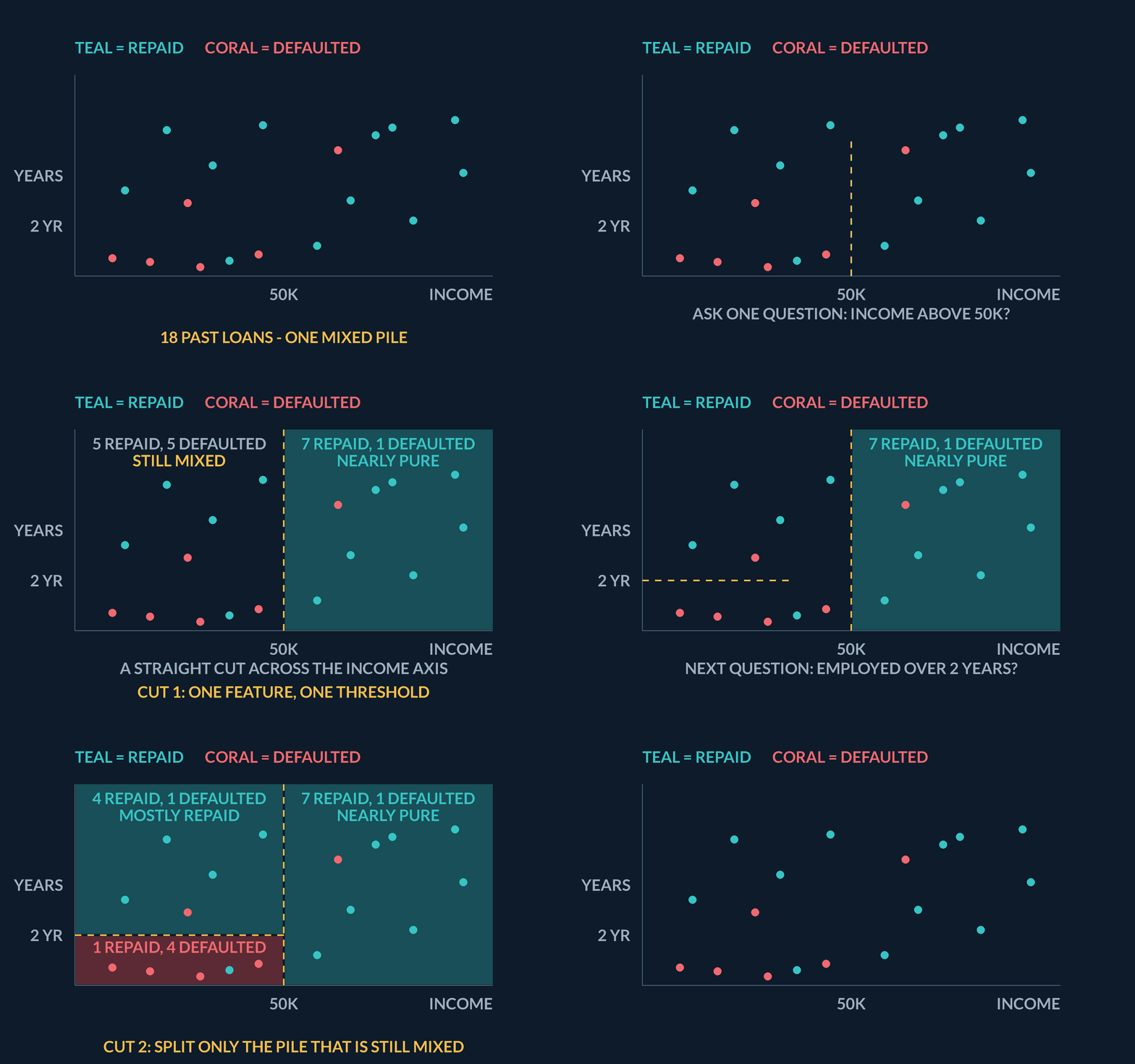
Two stacked cuts, scored by counting
The loan office plots 18 past applications by income and years employed: 12 repaid, 6 defaulted. The cut at income 50k puts 8 applications on the high-income side — 7 repaid, 1 defaulted — and leaves 10 on the low-income side, 5 repaid and 5 defaulted. A second cut at 2 years employed, drawn only across the low-income side, puts 5 of those applications above it — 4 repaid, 1 defaulted — and 5 at or below, 1 repaid and 4 defaulted. Each pile announces its majority label. Count the wrong announcements three times — before any cut, after the income cut alone, and after both cuts — and see what each straight cut actually bought.
- Baseline, no cuts at all: one pile of 18 with 12 repaid against 6 defaulted, so the majority announcement is "repaid" for everyone — and every defaulter is announced wrongly6 errors out of 18
- Bookkeeping check on the income cut before trusting it: repaid rows 7 + 5 = 12 and defaulted rows 1 + 5 = 6the two piles account for all 18 applications
- High-income pile after the cut: 7 repaid against 1 defaulted, majority says "repaid", and only the lone defaulter is announced wrongly1 error in its 8 rows
- Low-income pile: 5 repaid against 5 defaulted — dead even, so whichever label it announces, 5 of its 10 rows are wrong. The income cut alone therefore leaves 1 + 5 = 6 errors6 of 18 — the first cut alone scores no better than no tree
- Employment cut, across the low-income pile only: above 2 years the pile is 4 repaid against 1 defaulted, announcing "repaid" with 1 error; at or below it is 1 repaid against 4 defaulted, announcing "defaulted" with 1 errorthe mixed 10 becomes two piles of 1 error each
- Total for the finished three-leaf tree: 1 + 1 + 1 errors, against the baseline's 63 errors out of 18 — the stacked cuts halved the mistakes
Pro tip. Notice where the second cut runs: only across the low-income pile. A threshold in a tree slices the one pile it splits, never the whole plane — which is why tree regions come out as rectangles nested inside rectangles, and why the nearly-pure high-income pile is never charged for a question it does not need.
Why do standard decision trees produce orthogonal, rectangular decision regions in 2D feature space?
- Because tree algorithms require all features to be normalised to [0, 1]
- Because each internal node splits on a single feature against a scalar threshold
- Because leaf nodes can only output binary integer predictions
- Because pruning algorithms discard all diagonal gradient vectors
Splitting on one variable at a time (e.g., x <= 3) creates decision boundaries parallel to the coordinate axes, forming rectangular partitions.
3Gini, entropy, and greedy search
Gini and entropy are simply the two standard formulas for turning that mixed-ness into a number. You do not need to memorise either formula to use trees; what matters is that both give 0 for a pure pile, both peak at a 50/50 mix, and both fall as a pile gets more one-sided. When a library says it is splitting "by Gini", it just means: this is the ruler it holds up to each pile.
At each node the learner tries many candidate questions — every feature, many thresholds — and for each one measures how much the impurity would drop from the parent pile to the two child piles. It keeps the single question with the biggest drop, commits to it, and moves on. This strategy is called greedy: take the best cut available right now, with no looking ahead. Greedy search is fast and usually good enough for tabular data, but be clear about what it does not promise — it never compares whole trees against each other, so it is not guaranteed to find the globally best tree.
| Idea | Meaning |
|---|---|
| Pure node | All labels the same |
| Gini / entropy | How mixed the labels are |
| Greedy split | Best local cut, not global optimum |
Two candidate questions, one Gini ruler
Back at the loan stack: here is a tiny 8-row slice of it, each row written as (income in thousands, years employed, outcome): (60, 4, repaid), (55, 3, repaid), (72, 1, repaid), (40, 5, repaid), (45, 3, defaulted), (38, 1, defaulted), (30, 2, defaulted), (48, 1, defaulted). The learner is choosing the root question and has two candidates on the table: "income above 50?" and "employed more than 2 years?". Score both with Gini impurity G = 1 - \sum_k p_k^2 — where p_k is simply the fraction of a pile's rows belonging to class k — and keep the question with the bigger impurity drop.
- Parent pile, before any question: 4 repaid and 4 defaulted out of 8 rows, so both class fractions are 4/8 = 0.5. Gini: G = 1 - (0.5^2 + 0.5^2) = 1 - (0.25 + 0.25)G = 0.50 — the most mixed a two-class pile can be
- Candidate "income above 50?", yes pile: the rows earning 60, 55 and 72 — that is 3 repaid, 0 defaulted, so the fractions are 3/3 = 1 and 0/3 = 0. G = 1 - (1^2 + 0^2)G = 0 — a pure pile
- Its no pile: the five rows earning 50 or less — 1 repaid, 4 defaulted, fractions 1/5 = 0.2 and 4/5 = 0.8. G = 1 - (0.2^2 + 0.8^2) = 1 - (0.04 + 0.64)G = 0.32
- A split is scored by the weighted average of its children, each pile counting in proportion to its share of the 8 rows: (3/8)(0) + (5/8)(0.32) = 0 + 0.20. Drop from the parent: 0.50 - 0.20income question: drop = 0.30
- Candidate "employed more than 2 years?", yes pile: the rows with 4, 3, 5 and 3 years — 3 repaid, 1 defaulted, fractions 3/4 = 0.75 and 1/4 = 0.25. G = 1 - (0.75^2 + 0.25^2) = 1 - (0.5625 + 0.0625)G = 0.375
- Its no pile: the rows with 1, 1, 2 and 1 years — 1 repaid, 3 defaulted. Same two fractions the other way round, so the same arithmetic: G = 1 - (0.25^2 + 0.75^2)G = 0.375
- Weighted average for the employment split: (4/8)(0.375) + (4/8)(0.375) = 0.1875 + 0.1875 = 0.375. Drop from the parent: 0.50 - 0.375employment question: drop = 0.125
- Compare the drops: the income question removes 0.30 of impurity, the employment question only 0.125. The greedy learner keeps the bigger drop and commitsroot asks "income above 50?" — the same question at the top of this lesson's tree
Pro tip. Never judge a split by its prettiest-sounding child. The employment split feels tidy — two balanced piles of four — but the ruler is the weighted average, and the income question's 3-row pure pile plus a 0.32 pile average to 0.20, well below 0.375. This is also greedy search in miniature: two candidates scored, one kept, no looking ahead.
When constructing a decision tree, how is the best split chosen at a node?
- By running backpropagation with stochastic gradient descent across all branches
- By greedily evaluating candidate feature splits and picking the one that maximizes impurity reduction
- By selecting the split that maximizes tree depth on the training set
- By choosing randomly from the top 10% most variable input features
Decision tree induction evaluates all feature thresholds greedily at each step, picking the split that yields the greatest reduction in Gini impurity or entropy.
4Stopping before the tree memorises
Left unconstrained, the tree keeps splitting until every leaf is perfectly pure — and that is a trap, not a triumph. With enough depth, every quirky training row can earn its own private path and its own one-row leaf: the tree has memorised the training table, noise and all, and will answer confidently and wrongly on new rows. Perfect purity on the training data is often the signature of a tree that has stopped learning patterns and started photographing examples.
The first two knobs for stopping that are max_depth and min_samples_leaf. max_depth caps how many questions deep any path may go — depth 3 means at most three questions before an answer. min_samples_leaf refuses any split that would leave a leaf holding fewer than that many rows, so no leaf can be carved around a single odd example. Reach for these two before reaching for a hundred-tree ensemble.
One caveat to carry into the next lesson: impurity drop is a local score. A split that looks weak on its own — barely cleaning up the piles — can still be exactly the cut a later, stronger split depends on, and a greedy learner scoring one cut at a time cannot see that. This blind spot is one reason ensembles of many trees, coming up next, beat any single tree.
- Pick a split featureAt each node, choose the column and threshold that best separates the labels.
- Measure impurity dropGini or entropy scores how mixed the labels are — the best split maximises the drop.
- Stop before memorisingCap max_depth or min_samples_leaf so leaves hold enough rows to generalise.
| Setting | What happens | Why it matters |
|---|---|---|
| No limits at all | Splitting continues until every leaf is perfectly pure — quirky rows earn private one-row leaves | The tree photographs the training table, noise and all, and answers confidently and wrongly on new rows |
| max_depth | Caps how many questions deep any path may go — depth 3 means at most three before an answer | Cuts off the long private paths memorisation needs |
| min_samples_leaf | Refuses any split that would leave a leaf holding fewer than that many rows | No leaf can be carved around a single odd example |
Two stopping knobs applied to the loan tree
Take the finished loan tree of this lesson's cuts. The income question splits 18 applications into a high-income pile of 8 (7 repaid, 1 defaulted) and a low-income pile of 10 (5 repaid, 5 defaulted); the employment question then splits the low-income pile into 5 applications above 2 years (4 repaid, 1 defaulted) and 5 at or below (1 repaid, 4 defaulted). Each of its three leaves announces its majority label and makes exactly 1 error — 3 errors in 18. Now work the two stopping knobs on this exact tree: first cap max_depth at 1, then instead set min_samples_leaf to 3, and count what each rule allows, refuses, and costs.
- max_depth = 1 keeps only the income question, so the two low-income leaves (1 error each) merge back into one 5-against-5 pile where either announcement gets 5 wrong. The error count moves from 1 + 1 + 1 = 3 to 1 + 56 errors out of 18
- Compare that 6 to announcing "repaid" for all 18 with no tree at all, which wrongs exactly the 6 defaultersalso 6 — the depth cap threw away precisely the follow-up split that made the income cut pay off
- min_samples_leaf = 3, checked against the income cut: it makes children of 8 and 10 rows, and both are at least 3allowed
- Checked against the employment cut: children of 5 and 5 rows, both at least 3allowed — the full two-question tree stands under this rule
- Could growth continue below those leaves? Splitting a 5-row pile can only make children of 1-and-4 or 2-and-3 rows, and each shape has a side smaller than 3no legal split exists — both 5-row leaves are frozen
- The high-income leaf holds 8 rows including its single defaulter. The tempting split that carves that one quirky row into a private leaf makes a 1-row child, refused because 1 < 3; only 4-and-4 or 5-and-3 shapes stay legalthe memorising split is exactly the one the rule forbids
Pro tip. min_samples_leaf = 3 quietly outlaws more than tiny leaves: a pile needs at least 2 \times 3 = 6 rows before any split of it is legal, so every 5-row pile in this tree froze automatically. The knob is a stronger brake than its name suggests — it bounds which piles may split at all, not just how small a leaf may be.
A candidate split barely reduces impurity, so a classmate calls it useless anywhere in the tree. What does the lesson say?
- They are right: low impurity drop always means a useless split
- Impurity only matters at the root node
- Impurity drop is a local score — a split weak on its own can still matter if a later split needs it
- The tree search is global, so weak splits are never chosen
The learner is greedy and scores each cut locally. A weak-looking split can set up a strong later one — one reason ensembles of trees help.
5Lab: fit a shallow tree
This lab fits a real tree and then lets you look at what it learned. DecisionTreeClassifier is scikit-learn's ready-made tree learner, and max_depth=3 tells it: ask at most three questions along any path before you must give an answer. The data is a small made-up table of 400 rows with exactly two feature columns — two, on purpose, so that every row is just a point on a flat plane and the whole model can be drawn as a picture.
Read the variable names in Cell 1 before running it, because every one has a plain meaning. X is the table of feature values (each row one example, each column one feature) and y is the matching column of correct labels. train_test_split deals them into X_train and y_train — the rows the tree is allowed to learn from — and X_test and y_test, a held-out quarter the fit never sees. The printed score is accuracy on that held-out quarter, which is the honest number: scoring on rows the tree already studied would only tell you how well it memorised.
The two cells share one running Python kernel, like two paragraphs of the same notebook. Cell 1 leaves model, X_train, and y_train alive in that kernel; Cell 2 simply reuses them. So after the fit, you can tweak the plot title or the mesh size and re-run only Cell 2 — no refitting needed.
Cell 2 paints the tree's decision regions, and the trick is worth understanding: it lays a fine grid of points (the mesh built by meshgrid) across the whole plane, asks the fitted tree to predict a class for every grid point, and colours each point by the answer. The coloured patches that emerge should look blocky — rectangles with straight vertical and horizontal edges — and that blockiness is the previous concept made visible: each split cuts one feature at one threshold, so every boundary the tree can draw is a straight axis-aligned line.
Now break it on purpose. Raise max_depth to something large without raising min_samples_leaf, re-run both cells, and watch the regions fragment into tiny islands wrapped around individual training dots. Each little island is a leaf carved for one quirky row — memorisation you can literally see. If the train score climbs while the held-out score sinks, you are watching overfitting happen in real time.
No diagram — the fit is drawn by the coding lab plot, not a static figure.
| Step | Why |
|---|---|
| Hold out a test fold | Score must use rows the fit never saw |
| Cap max_depth | Unbounded depth memorises the train table |
| Paint decision regions | Axis-aligned blocks show what the tree actually learned |
Coding lab. Shallow decision tree runs in the app, with checks on your output.
You raise max_depth without raising min_samples_leaf and the painted regions fragment into tiny patches around single training points. What are you looking at?
- The tree discovering fine real structure in the data
- Memorisation you can see — leaves carved around individual quirky rows
- A rendering artifact of the mesh in the plot cell
- Proof that the two features are collinear
Unconstrained depth lets every quirky row earn its own leaf. Tiny single-point regions are the visual signature of an overfit tree.
Notes
- A decision tree asks a sequence of feature questions and sends each row down a branch until a leaf predicts the label.
- Gini and entropy score how mixed the labels are inside a node; a pure leaf (all one class) scores best.
- First knobs: max_depth and min_samples_leaf — raise leaf size or cut depth before you reach for a hundred-tree ensemble.
Exam traps & shortcuts
- Keep lab datasets under 2000 rows in the browser runtime.
- Split train and test before fitting any model that sees labels.
Recap
This lesson in brief:
- Decision trees
- A decision tree asks a sequence of feature questions and sends each row down a branch until a leaf predicts the label.
- Impurity and splits
- Gini and entropy score how mixed the labels are inside a node; a pure leaf (all one class) scores best.
- Depth knobs
- First knobs: max_depth and min_samples_leaf — raise leaf size or cut depth before you reach for a hundred-tree ensemble.
Practise Decision Trees
Reading is free and needs no account. Practice, mocks and progress live in the app.
- 10 exam-style questions on this topic, with explanations
- A 5-question practice set that ends the chapter
- Timed mocks scored with the real marking scheme
- Readiness tracked per topic, kept on your device