Machine Learning · Machine Learning Core
Boosting
Boosting stacks trees in sequence so each new model chases residual errors — powerful on tabular data, and easy to overfit if you never early-stop.
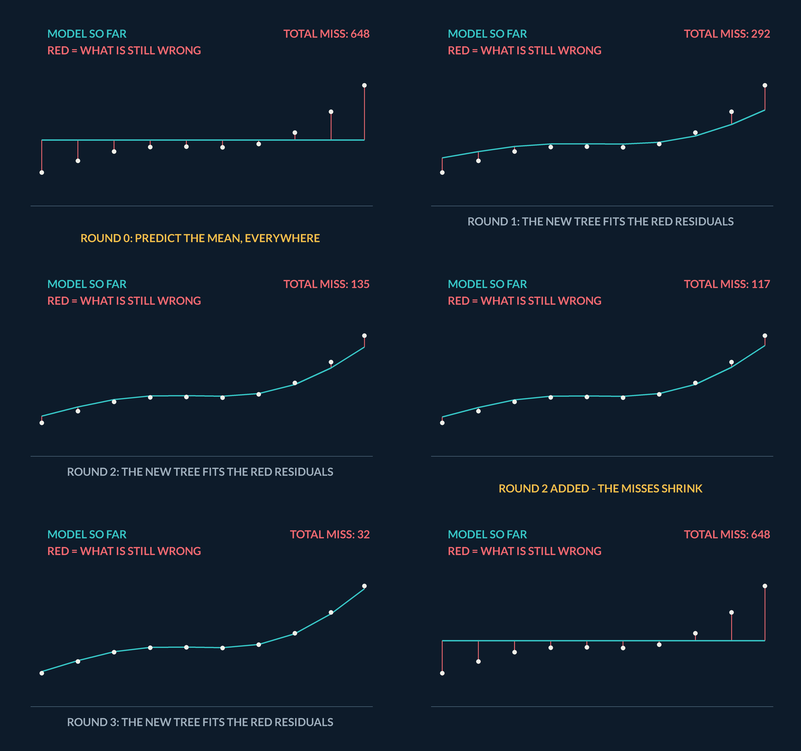
Bagging averages independent trees; boosting builds a sequence. Each new tree is fitted against what the current ensemble still gets wrong, so residuals shrink round by round — and keep shrinking into noise if you never stop. This lesson locks that intuition, then fits a histogram gradient booster in the browser and compares it to a simple baseline.
- Machine Learning
- Medium level
- 4 concepts
- 10 practice questions
1Boosting intuition
Imagine you and three friends are guessing house prices. You go first, and you keep it simple: you guess the neighbourhood average for every single house. Some guesses land close, others miss badly — one house sells for far more than your guess, another for a little less. Now here is the trick: your first friend does not start over from scratch. Instead, she looks only at how much you missed each house by, and tries to predict those misses. The next friend then looks at whatever error is still left after her correction, and predicts that. Each person's whole job is to fix what the people before them got wrong.
That guessing game is boosting. Each guesser is called a weak learner — 'weak' because on its own it is only slightly better than a blind guess. In practice the weak learner is usually a very shallow decision tree, sometimes just one yes/no question deep. The whole team together — your average guess plus every friend's correction stacked on top — is called the ensemble, which is just the word for the combined model. The ensemble's prediction for a house is your guess plus friend one's correction plus friend two's correction, and so on down the line.
Figure. Each weak learner's whole job is to fix what the guessers before it got wrong: the ensemble's prediction is the first guess plus every friend's correction stacked on top of it.
| In the guessing game | ML name | What it contributes |
|---|---|---|
| You, guessing the neighbourhood average for every house | The starting model | A simple first guess — close on some houses, badly off on others |
| Each friend, predicting only how much the guessers before her missed | Weak learner | A very shallow tree, sometimes one yes/no question deep — alone, only slightly better than a blind guess |
| The whole team's stacked answer | The ensemble | Your guess plus every friend's correction added on top, down the line |
The guessing game, played once at full strength
Play one round of the team-of-friends game on the four-house street that runs through this topic. The houses' true selling prices are y = [2, 3, 7, 2], in crores of rupees. You go first and, exactly as the game says, you guess the neighbourhood average for every single house. Then friend 1 takes her turn: her job is not to re-guess prices but to predict your misses — how far each house's true price sits from your guess. She is a weak learner one yes/no question deep: she asks 'is it two-storey?' (houses 2 and 3 are the street's only two-storey houses) and answers with the average miss of the houses in each of her two groups. Apply her correction at full strength — no holding back — and see what the team's stacked answer looks like.
- Your first guess, the neighbourhood average: (2 + 3 + 7 + 2) ÷ 43.5 crore for every house
- Your misses, house by house (true price minus your guess): 2 − 3.5, 3 − 3.5, 7 − 3.5, 2 − 3.5[−1.5, −0.5, +3.5, −1.5]
- Friend 1 asks 'is it two-storey?'. Her two-storey group holds houses 2 and 3, so her correction there is their average miss: (−0.5 + 3.5) ÷ 2+1.5
- Her single-storey group holds houses 1 and 4: (−1.5 + (−1.5)) ÷ 2−1.5
- The team's stacked answer — your guess plus her correction: [3.5 − 1.5, 3.5 + 1.5, 3.5 + 1.5, 3.5 − 1.5][2, 5, 5, 2]
- The leftover misses friend 2 would inherit: [2 − 2, 3 − 5, 7 − 5, 2 − 2][0, −2, +2, 0]
- Total miss size, before and after her turn: 1.5 + 0.5 + 3.5 + 1.5, then 0 + 2 + 2 + 07 → 4
Pro tip. Notice what one full-strength turn did: houses 1 and 4 became perfect, but house 2 — which your average missed by only 0.5 — got dragged 2 too high, because it shares a two-storey answer with badly-missed house 3 and a one-question friend can only give one correction per group. The team still improved (total miss 7 down to 4), yet one house is now worse than before its 'correction'. That shared-answer overshoot is exactly why real boosters shrink every correction with a learning rate before adding it.
How does the fundamental training strategy of boosting differ from random forests (bagging)?
- Boosting fits deep trees in parallel while bagging fits shallow stumps sequentially
- Boosting ignores training labels while bagging optimizes log loss directly
- Boosting trains trees sequentially to correct the residuals of prior trees, whereas bagging trains trees independently in parallel
- Boosting requires all features to be continuous while bagging handles only text
Bagging fits independent trees in parallel on bootstrap samples. Boosting builds an iterative sequence where each learner repairs the errors of the preceding ones.
2Residuals drive the sequence
The 'how much did we miss by' number has a name too: the residual. If a house actually sold for y (the true answer) and the team's current combined guess is \hat{y} (read 'y-hat', the prediction), the residual is r = y - \hat{y} — simply true value minus predicted value, the leftover mistake. A residual of zero means that house is already predicted perfectly; a big residual means the team is still badly wrong there. Each new tree in the sequence is trained with these residuals as its targets, so it naturally spends its effort on the houses the team is missing worst.
This is the key difference from bagging, the ensemble method where many trees are trained independently on random samples and their answers averaged. Bagging's trees never talk to each other — each one tries to solve the whole problem alone. Boosting's trees are the opposite: they form a sequence, and tree number ten is meaningless without trees one through nine, because ten was trained purely to patch their remaining mistakes. This is called sequential correction, and it is why boosting can drive errors down so fast.
| Question | Bagging | Boosting |
|---|---|---|
| How the trees are trained | Independently, each on a random sample of rows | In sequence — each new tree takes the residuals r = y - \hat{y} as its targets |
| Do the trees talk to each other? | Never — each tries to solve the whole problem alone | Always — tree ten is meaningless without trees one through nine |
| How the answers combine | Their answers are averaged | Each tree patches the mistakes still left, so errors drop fast — sequential correction |
What the next tree trains on — and what a bagged tree would see
Same four-house street: true prices y = [2, 3, 7, 2] in crores of rupees, and the team's current combined guess is the round-0 stump that predicts 2 for every house. Boosting's next tree never sees prices as its targets — it trains on the residuals r = y - \hat{y}, the leftover mistakes. Compute those targets and measure where the miss is concentrated. Then run the bagging contrast with numbers: a bagged tree instead gets a bootstrap resample of the street — four draws with replacement from the four houses, original prices as its targets — so some houses repeat and some are left out entirely. Work out how likely such a resample is to leave out house 3, the house the team misses worst.
- The next tree's training targets, house by house: 2 − 2, 3 − 2, 7 − 2, 2 − 2[0, 1, 5, 0]
- Total miss size: 0 + 1 + 5 + 0 = 6, of which house 3 carries 5 ÷ 6≈ 0.83 — 83% of the target mass sits on house 3
- Bagging contrast — one perfectly ordinary resample draws house 1, house 1, house 2, house 4, so that tree's target column is the original prices [2, 2, 3, 2]house 3 never appears
- How often does that happen? Each draw picks one of 4 houses, so a single draw misses house 3 with chance 3 ÷ 4; all four draws miss it with chance (3/4) × (3/4) × (3/4) × (3/4) = 81 ÷ 256≈ 0.32
- Put the two side by side: chance a bagged tree never sees the worst-missed house, versus the share of the boosted tree's targets staked on itabout 1 in 3, versus 83%
Pro tip. The residual column [0, 1, 5, 0] is not a shrunken copy of the price column [2, 3, 7, 2] — houses 1 and 4 cost 2 crores yet contribute a target of exactly zero, because being predicted right, not being cheap, is what earns a zero. A tree trained on residuals is answering a different question ('where is the team still wrong?') than a bagged tree trained on prices ('what do houses cost?'), and that question changes every round as the mistakes shrink.
In boosting, what does the tree added at round n + 1 actually fit?
- A fresh bootstrap sample, independent of every earlier tree
- The residual errors the current ensemble still makes on the training rows
- The rows the first tree classified correctly
- The validation fold, to keep the ensemble honest
Boosting is sequential: each new tree chases what the ensemble so far still gets wrong. That is the core difference from bagging's independent, bootstrap-grown trees.
3Small steps, and when to stop
There is one more dial to name: the learning rate. Rather than adding each friend's correction at full strength, the team only applies a fraction of it — typically 5% to 10%, written as a learning rate of 0.05 to 0.1. Why hold back? Because a friend who overreacts to one weird house would drag the whole team's guess off course. Shrinking every correction means no single round can dominate; the team takes many small, careful steps instead of a few reckless ones. Smaller steps need more rounds, but the progress is steadier.
Now the danger, and it follows directly from the story. The team never runs out of residuals: even when the real pattern is fully captured, every house still misses by a little bit of random noise — the seller was in a hurry, the photos were bad. If you keep adding correctors forever, they start memorising that noise, and the model becomes brilliant on the houses it trained on and worse on new ones. That is overfitting. The guard rail is to keep a set of held-out examples the training never sees, watch the score on them after each round, and stop adding rounds the moment that score stops improving — a practice called early stopping. In code you also cap the number of rounds directly (the parameter is usually called n_estimators or max_iter, literally 'how many trees to add').
- Start with a weak fitFirst model is shallow — it captures only the broadest pattern.
- Focus on residualsEach new tree targets the errors the ensemble still makes on train.
- Add with a learning rateShrink each tree's contribution so later rounds refine without overwriting earlier signal.
| Step | What happens |
|---|---|
| Fit a weak learner | A shallow tree that is only slightly better than chance |
| Up-weight misses | Next tree focuses on rows the ensemble still gets wrong |
| Add and stop | Sum the trees; stop when hold-out stops improving |
Two correction rounds by hand, with the brake on
Four houses sold for y = [2, 3, 7, 2] (prices in crores of rupees), and the round-0 stump predicts 2 for every house: \hat{y} = [2, 2, 2, 2]. The leftover mistakes are the residuals r = y - \hat{y} = [0, 1, 5, 0] — houses 1 and 4 are already right, house 2 is missed by 1, house 3 by 5. Houses 2 and 3 are the only two-storey houses, and 'is it two-storey?' is the one question each corrector stump can ask; a stump answers its question and outputs the average residual of the houses in each of its two leaves. Run two correction rounds with the learning rate set to 0.1 — every prediction moves by 0.1 times its leaf's output, not the full amount — and watch what the residuals do.
- Tree 1 fits the residuals [0, 1, 5, 0]. Its two-storey leaf holds houses 2 and 3, so it outputs their average residual: (1 + 5) ÷ 23
- Its other leaf holds houses 1 and 4, both already perfect: (0 + 0) ÷ 20
- Apply the brake before adding: the two-storey correction is scaled to 0.1 × 3+0.3
- Predictions after round 1: [2, 2 + 0.3, 2 + 0.3, 2][2, 2.3, 2.3, 2]
- Residuals after round 1: [2 − 2, 3 − 2.3, 7 − 2.3, 2 − 2][0, 0.7, 4.7, 0]
- Tree 2 fits [0, 0.7, 4.7, 0] with the same question. Two-storey leaf: (0.7 + 4.7) ÷ 2 = 2.7, braked to 0.1 × 2.7+0.27
- Predictions after round 2: [2, 2.3 + 0.27, 2.3 + 0.27, 2], so residuals [0, 3 − 2.57, 7 − 2.57, 0] = [0, 0.43, 4.43, 0][2, 2.57, 2.57, 2]
- Total miss, adding the residual sizes each round: 0 + 1 + 5 + 0, then 0 + 0.7 + 4.7 + 0, then 0 + 0.43 + 4.43 + 06 → 5.4 → 4.86
Pro tip. Rerun round 1 at full strength (learning rate 1) and the shared leaf adds the whole 3 to both two-storey houses: house 3 improves to a residual of 2, but house 2 — which was only 1 away — is dragged to a prediction of 5, an error of 2 and worse than before the 'correction'. The 0.1 brake keeps the shared step small enough that every residual it touches shrinks: house 2 goes 1 → 0.7 → 0.43, never overshooting. That steadiness is what more rounds buy — and since the residuals shrink but never reach zero, the stop signal is a stalling validation score, not an empty residual column.
Why does gradient boosting multiply each tree output by a small learning rate (e.g. 0.05)?
- It ensures the tree depth can be expanded to infinity without memory leaks
- It normalises the target variable so all residuals sum to zero
- Shrinking each step leaves room for future trees to refine predictions, improving generalisation and preventing rapid overfit
- It forces all tree split thresholds to fall between zero and one
A small learning rate (shrinkage) dampens each tree contribution, forcing the ensemble to learn gradually and generalise better.
4Lab: fit a booster
Time to run the guessing game for real. This lab builds a small fake dataset — 600 rows, each row an 'example' with 8 measured numbers (the features) and a label saying which of two classes it belongs to — and then trains a booster to predict the label from the numbers. The data comes from scikit-learn's make_classification helper, which invents a table with a genuine hidden pattern in it, so there is truly something for the model to learn.
Cell 1 does three things, in order, and each matters. First it splits the table: 75% of the rows become the training set the model is allowed to study, and 25% are locked away as the test set — rows the model will never see during fitting. This split must happen before any fitting, because a model scored on rows it already studied is like grading a student on the exact questions they rehearsed: the score tells you nothing about new data. Second, it fits a HistGradientBoostingClassifier — scikit-learn's fast gradient booster, the sequential fix-the-last-mistake machine from the previous concept. Its max_iter=50 means 'add at most 50 corrector trees', and learning_rate=0.1 means 'apply each tree's correction at one-tenth strength', exactly the two safety dials named earlier. Third, it scores the fitted model on the held-out test rows and prints that number: the fraction of unseen rows classified correctly.
Cell 2 answers the question a raw score cannot: is that number actually good? Suppose 60% of the rows belong to class A. A 'model' that ignores the features entirely and shouts 'A!' every time already scores 60%. scikit-learn packages that lazy strategy as DummyClassifier(strategy="most_frequent") — the majority-class baseline. Cell 2 fits it, scores it on the same test rows, and draws both scores side by side as a bar chart. The booster only deserves credit for the gap between its bar and the dummy's bar; a booster that merely matches the baseline has learned nothing from the features.
Two practical notes on the lab itself. The cells share one running Python session (the kernel), so the model and the train/test splits created in Cell 1 are still alive when Cell 2 runs — that is why Cell 2 can use them without redefining anything, and why you can tweak Cell 2's colours or title and re-run just that cell. And keep n_samples in the hundreds: everything here runs inside your browser, and a few hundred rows keeps the fit snappy while being plenty to see boosting beat the baseline.
No diagram — the score comparison is drawn by the coding lab plot, not a static figure.
| Step | Why |
|---|---|
| Hold out a test fold | Score must use rows the fit never saw |
| Fit HistGradientBoostingClassifier | Sequential trees chase residual errors |
| Bar-plot vs DummyClassifier | A majority baseline shows whether boosting earned its lift |
Coding lab. Fit a histogram gradient booster runs in the app, with checks on your output.
Why does the lab bar the booster's hold-out score against a majority-class DummyClassifier instead of just printing it?
- DummyClassifier is a stronger booster with different defaults
- sklearn requires a baseline model in every pipeline
- A booster that only matches the majority baseline has learned nothing — the baseline shows whether the lift is real
- The dummy's score calibrates the plot's y-axis automatically
On an imbalanced table a bare score can look fine while equalling the majority vote. The dummy baseline is the floor any real learning must clear.
Notes
- Boosting adds models in sequence; each new tree focuses on the residual errors the current ensemble still makes.
- Unlike bagging, the trees are not independent — later rounds explicitly chase what earlier rounds missed.
- Watch validation curves and early-stop (or limit n_estimators / learning rate) before trusting a boosted score on the test fold.
Exam traps & shortcuts
- Keep lab datasets under 2000 rows in the browser runtime.
- Split train and test before fitting any model that sees labels.
Recap
This lesson in brief:
- Sequential repair
- Boosting adds models in sequence; each new tree focuses on the residual errors the current ensemble still makes.
- Dependent learners
- Unlike bagging, the trees are not independent — later rounds explicitly chase what earlier rounds missed.
- Early stop
- Watch validation curves and early-stop (or limit n_estimators / learning rate) before trusting a boosted score on the test fold.
Practise Boosting
Reading is free and needs no account. Practice, mocks and progress live in the app.
- 10 exam-style questions on this topic, with explanations
- A 5-question practice set that ends the chapter
- Timed mocks scored with the real marking scheme
- Readiness tracked per topic, kept on your device