Machine Learning · Machine Learning Core
k-means Clustering
Group similar rows without labels: k-means assign-and-move, when the geometry fails, and a browser lab that fits and scatters clusters.
Not every useful table has a label. This lesson locks k-means for grouping similar rows — how the assign-and-move loop works, when the geometry lies, and a notebook that fits and scatters three blobs.
- Machine Learning
- Medium level
- 5 concepts
- 10 practice questions
1Where should the kitchens go
Start with a picture you already know. A food-delivery company wants to open three kitchens in a city, and it has a map with a dot for every customer's house — 300 dots. Where should the three kitchens go so that every house is reasonably close to one of them? Nobody has labelled the houses "north group" or "south group"; the dots are just dots. Finding good kitchen spots, and deciding which houses belong to which kitchen, is exactly the problem k-means solves.
Two words before anything runs. Each house is a point: one row of your data table, drawn at the position its numbers describe. A kitchen is a centroid: an ordinary point that marks the centre of one group — it is not a data point itself, just a marker the algorithm is free to move around. And k is simply how many centroids you ask for. In the kitchen story k = 3 because the company decided on three kitchens. You pick that number before the algorithm runs; k-means never picks it for you.
| Word | Meaning |
|---|---|
| Point | One row of your table, drawn at the position its numbers describe |
| Centroid | A movable marker for the centre of one group - not a data point itself |
| k | How many centroids you ask for - you pick it before the algorithm runs |
What objective does the k-means clustering algorithm attempt to minimise?
- The sum of squared Euclidean distances between each data point and its assigned cluster centroid
- The maximum geometric margin separating two supervised classification classes
- The cross-entropy loss computed against ground-truth categorical labels
- The total number of input features retained after projection
k-means minimizes inertia (within-cluster sum of squares).
2Assign, move, repeat
The algorithm starts by dropping its k centroids somewhere — often at random, so the first guesses are usually bad. Then comes the assignment step: every house looks at all three kitchens, measures the straight-line distance to each, and joins the closest one. After this step every point carries a group label — "I belong to kitchen 2" — even though nothing has been optimised yet.
Next comes the update step, and this is where the name k-MEANS comes from. Each kitchen looks at the houses that just joined it and moves to their mean — the plain average of their positions (average all their horizontal coordinates to get the new horizontal position, and the same for vertical). Averaging drags every kitchen into the middle of its own neighbourhood, which is obviously a better spot than the random one it started at.
But wait — once the kitchens have moved, some houses might now be closer to a different kitchen than the one they joined. So the algorithm assigns again, then averages again, and keeps alternating: assign, move, assign, move. It stops when a full pass changes nothing — no house switches kitchens, so no kitchen moves — or when an iteration budget runs out. That standstill is what "the algorithm converged" means.
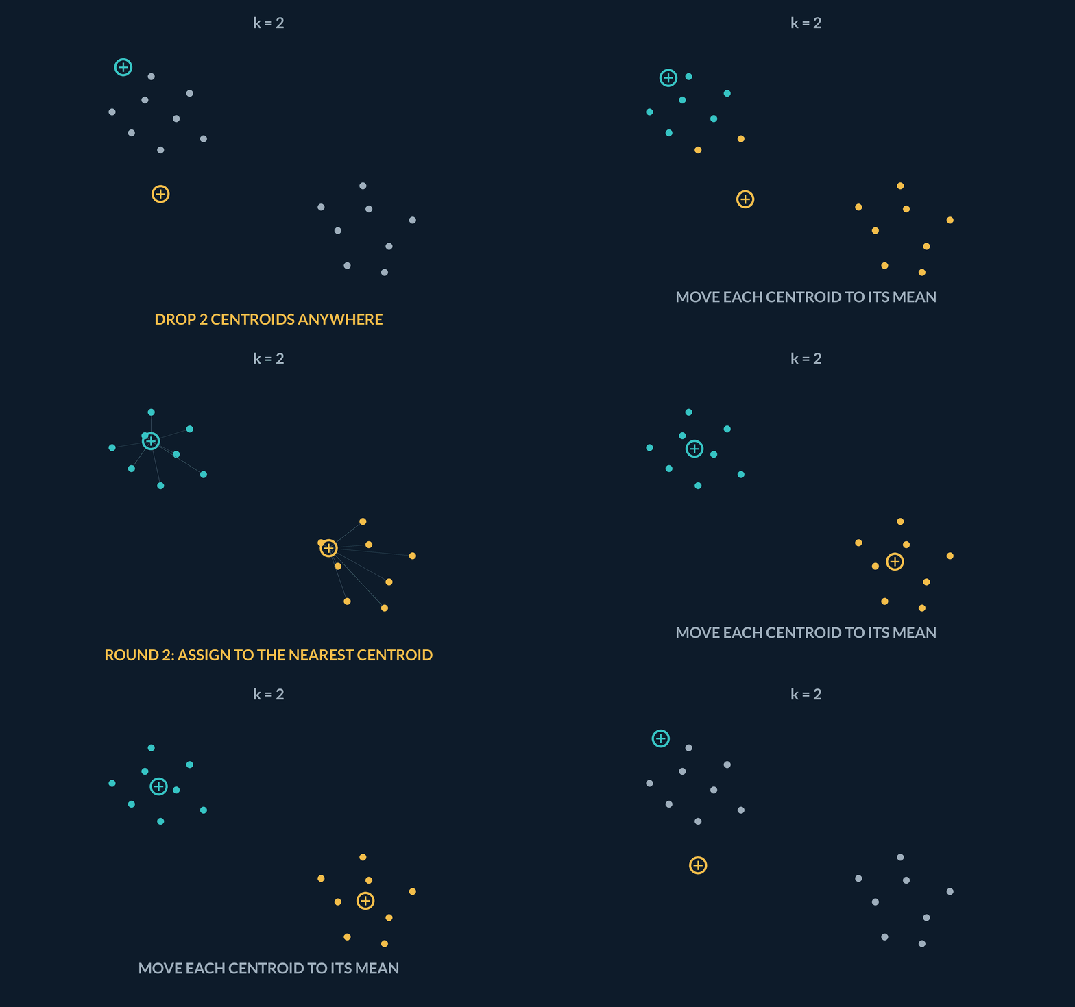
- Choose kDecide how many groups you want before the algorithm runs — three kitchens means k = 3. Elbow plots, silhouette scores, and domain knowledge guide the number; the data will never volunteer it, and peeking at the labels afterwards to justify a k is circular.
- Assign to nearest centroidEvery point measures its distance to all k centroids and joins the closest one — each house picks its nearest kitchen. After this pass, every row carries a group label, even on the very first, still-random round.
- Update and repeatMove each centroid to the mean — the plain average position — of the points that joined it, which drags it into the middle of its own group. Then assign again, because the move may have changed which centre is nearest. Stop when a full pass changes no label.
| Step | Working | Result |
|---|---|---|
| Assign to K1 (0, 0) | H1, H2, H3 — squared gaps 2, 4, 4 (vs 82, 64, 104 to K2) | K1's group: H1, H2, H3 |
| Assign to K2 (10, 0) | H4, H5, H6 — squared gaps 2, 4, 4 (vs 82, 104, 64 to K1) | K2's group: H4, H5, H6 |
| Move K1 to its mean | east (1 + 2 + 0) ÷ 3 = 1, north (1 + 0 + 2) ÷ 3 = 1 | K1 moves (0, 0) → (1, 1) |
| Move K2 to its mean | east (9 + 10 + 8) ÷ 3 = 9, north (1 + 2 + 0) ÷ 3 = 1 | K2 moves (10, 0) → (9, 1) |
| Assign again | H3, nearest the boundary: squared gap 2 to moved K1, 82 to K2 — stays; so do the rest | No house switches → converged |
One full round by hand: six houses, two kitchens
A pilot run on one street of the delivery map. Two trial kitchen spots: K1 at (0, 0) and K2 at (10, 0) — every pair of numbers is a position in km east and km north of the depot. Six houses: H1 at (1, 1), H2 at (2, 0), H3 at (0, 2), H4 at (9, 1), H5 at (10, 2), H6 at (8, 0). Run one full round by hand: assign every house to its nearest kitchen, then move each kitchen to the mean of its houses. One shortcut before we start: nearest is nearest whether you compare distances or squared distances, so each row below computes the squared distance — the east gap squared plus the north gap squared — and skips every square root.
- H1 to K1: (1−0)² + (1−0)² = 1 + 1 = 2; H1 to K2: (1−10)² + (1−0)² = 81 + 1 = 822 < 82 → joins K1
- H2 to K1: (2−0)² + (0−0)² = 4 + 0 = 4; H2 to K2: (2−10)² + (0−0)² = 64 + 0 = 644 < 64 → joins K1
- H3 to K1: (0−0)² + (2−0)² = 0 + 4 = 4; H3 to K2: (0−10)² + (2−0)² = 100 + 4 = 1044 < 104 → joins K1
- H4 to K1: (9−0)² + (1−0)² = 81 + 1 = 82; H4 to K2: (9−10)² + (1−0)² = 1 + 1 = 22 < 82 → joins K2
- H5 to K1: (10−0)² + (2−0)² = 100 + 4 = 104; H5 to K2: (10−10)² + (2−0)² = 0 + 4 = 44 < 104 → joins K2
- H6 to K1: (8−0)² + (0−0)² = 64 + 0 = 64; H6 to K2: (8−10)² + (0−0)² = 4 + 0 = 44 < 64 → joins K2
- Update K1 — the mean of its three houses H1, H2, H3: east (1 + 2 + 0) ÷ 3 = 1, north (1 + 0 + 2) ÷ 3 = 1K1 moves to (1, 1)
- Update K2 — the mean of H4, H5, H6: east (9 + 10 + 8) ÷ 3 = 9, north (1 + 2 + 0) ÷ 3 = 1K2 moves to (9, 1)
- Assign again from the moved kitchens — checking H3, the house nearest the boundary: to K1 at (1, 1) it is (0−1)² + (2−1)² = 1 + 1 = 2, to K2 at (9, 1) it is (0−9)² + (2−1)² = 81 + 1 = 82, so it stays with K1; the other five stay put the same wayno house switches → converged
Pro tip. Skipping the square root is not laziness — the root never changes which kitchen is nearest, and dropping it is exactly what fast implementations do. Just never report a squared value as a distance: H1's squared gap to K2 is 82, but the straight-line distance is √82 ≈ 9.1 km. And this round only converged immediately because the two house groups sit far apart; on real data the loop usually needs several assign-and-move rounds before a full pass changes nothing.
During one iteration of k-means, what happens in the 'update' step after all points are assigned?
- The value of k is incremented by one to capture leftover unassigned points
- Each centroid is relocated to the arithmetic mean position of all data points currently assigned to it
- All data points are shifted to the origin of the coordinate space
- The distance metric is switched from Euclidean to Manhattan distance
In the update step, each centroid is recalculated as the center of mass (mean) of all points currently assigned to that cluster.
3Choosing k, and a scaling trap
Notice what you decided and what the data decided. You chose k; the data only chose where the k centres settled. There is no free correct k the algorithm hands back. Silhouette scores — a number per point measuring how snugly it sits in its own group compared to the nearest other group — plus domain knowledge ("marketing wants three actionable segments") are what guide the choice.
One trap to disarm before you ever run it: distance only means what you want it to mean if the columns are on comparable scales. Cluster customers on yearly income in rupees (differences in the tens of thousands) and age in years (differences of five or ten), and the income gaps utterly dominate every distance — you have built an income sorter that ignores age. Scale the features to similar ranges first, whenever the columns live on different units.
Figure. Cluster on raw income (differences in the tens of thousands of rupees) next to age (differences of five or ten years) and the income gaps utterly dominate every straight-line distance - you have built an income sorter that ignores age. Scale the features to similar ranges first.
The 35-year age gap that lost to Rs 2,000
The delivery company now clusters customers instead of houses. Each customer is a point with two coordinates: yearly income in rupees and age in years. Three customers — A earns Rs 40,000 at age 25; B earns Rs 42,000 at age 60; C earns Rs 60,000 at age 26. Who is A's nearest neighbour? Use the same shortcut as always: nearest is nearest whether you compare distances or squared distances, so each row computes the squared distance — the income gap squared plus the age gap squared — and skips every square root. Do it twice: first on the raw numbers, then after putting both columns on comparable footing by dividing every income by a typical income spread of Rs 10,000 and every age by a typical age spread of 10 years.
- Raw A to B: income gap 42,000 − 40,000 = 2,000, squared 4,000,000; age gap 60 − 25 = 35, squared 1,225; total 4,000,000 + 1,2254,001,225
- Raw A to C: income gap 60,000 − 40,000 = 20,000, squared 400,000,000; age gap 26 − 25 = 1, squared 1; total400,000,001
- Raw verdict: 4,001,225 < 400,000,001, and the 35-year age gap contributed only 1,225 of A-to-B's 4,001,225 — a share of about 0.03%A's nearest neighbour is B, a 60-year-old
- Scale both columns: incomes ÷ 10,000 and ages ÷ 10 turn A into (4.0, 2.5), B into (4.2, 6.0), C into (6.0, 2.6)all coordinates now single digits
- Scaled A to B: (4.2 − 4.0)² + (6.0 − 2.5)² = 0.04 + 12.2512.29
- Scaled A to C: (6.0 − 4.0)² + (2.6 − 2.5)² = 4 + 0.014.01
- Scaled verdict: 4.01 < 12.29 — same three people, only the units changedA's nearest neighbour is now C, the near-twin in age
Pro tip. k-means never sees your intent, only coordinates — every assign step in the loop runs exactly this arithmetic against each centroid, so an unscaled income column quietly turns the whole clustering into an income sort that files a 25-year-old next to a 60-year-old. Real pipelines standardise each column (subtract its mean, divide by its spread); dividing by a stated typical spread, as here, is the same idea by hand.
A dataset has income in rupees (20,000 to 200,000) and age in years (18 to 70). What happens if you run k-means without scaling?
- The algorithm will fail to converge and produce a division-by-zero error
- Distance calculations will be overwhelmingly dominated by income, effectively ignoring age entirely
- Age will dominate the clustering because smaller numbers have larger gradients
- The number of clusters k will automatically collapse to 1
Euclidean distance squares differences. A difference of 5,000 rupees completely eclipses a 10-year age difference, so unscaled clustering only clusters on income.
4k groups, even from nothing
k-means also has a shape it likes. Because each group is "whatever is nearest to one centre", the happy case is compact, roughly round blobs of similar spread. Two nested rings, long stretched-out streaks, or one dense clump next to one sparse cloud all break the geometry: the centroids settle somewhere, but the boundaries they draw cut straight through the real structure.
And here is the quietest failure of all: k-means always returns exactly k groups, even when the data has no clusters whatsoever. Feed it a perfectly uniform cloud with k = 4 and it will dutifully slice the cloud into four tidy pieces and hand you four labels. Getting k labels back is not evidence that k groups exist — the algorithm was never allowed to answer "zero".
So before treating the labels as real segments, always plot a sample or read the cluster profiles (average income, average age, group sizes) and ask whether the groups make sense. If the shapes look wrong, reach for a different algorithm or transform the features — do not try to "fix" bad geometry by raising k forever.
| Situation | What goes wrong |
|---|---|
| Elongated / nested shapes | Centroids sit in the wrong place |
| No real clusters | Still emits k labels |
| Unscaled columns | One unit dominates distance |
Ask for 2 groups, then 3, on a road with none
Six houses stand along one straight road at km marks 1, 2, 3, 4, 5, 6 from the depot — perfectly evenly spaced, no clumps whatsoever. On a single road, the distance between a house and a kitchen is just the gap between their km marks. Run k-means twice on exactly this data: once with k = 2, dropping trial kitchens at marks 2 and 5, and once with k = 3, dropping trial kitchens at marks 1.5, 3.5 and 5.5. Watch what it hands back each time.
- k = 2, assign: house 1 is 1 km from K1 (at mark 2) and 4 km from K2 (at mark 5), so it joins K1; house 2 (gaps 0 vs 3) and house 3 (gaps 1 vs 2) join K1; houses 4, 5, 6 (gaps 2 vs 1, 3 vs 0, 4 vs 1) join K2K1: {1, 2, 3}, K2: {4, 5, 6}
- k = 2, move each kitchen to the mean of its houses: (1 + 2 + 3) ÷ 3 = 2 and (4 + 5 + 6) ÷ 3 = 5neither kitchen moves
- A full pass changed nothing, so the loop stopsconverged: two tidy groups
- k = 3 on the same road, assign: house 1 sits 0.5, 2.5 and 4.5 km from the three kitchens, so it joins K1; house 2 (0.5 vs 1.5 vs 3.5) joins K1; houses 3 and 4 (each 0.5 km from the kitchen at 3.5) join K2; houses 5 and 6 (each 0.5 km from the kitchen at 5.5) join K3K1: {1, 2}, K2: {3, 4}, K3: {5, 6}
- k = 3, move to the means: (1 + 2) ÷ 2 = 1.5, (3 + 4) ÷ 2 = 3.5, (5 + 6) ÷ 2 = 5.5no kitchen moves — converged: three tidy groups
- One structureless, perfectly even road: ask for 2 groups and get 2; ask for 3 and get 3k labels back is not evidence of k groups
Pro tip. Convergence is not endorsement. The loop stops when nothing moves, and here it stopped instantly both times — on data with zero cluster structure. Before believing the labels, look at where the boundaries fell: between houses 3 and 4 (or 2 and 3, and 4 and 5) the road is exactly as dense as everywhere else, which is the giveaway that the groups were sliced, not found. Group profiles and silhouette scores exist to catch precisely this.
You run k-means with k = 4 and get four groups, and a classmate concludes the data has four natural clusters. Why is that unsafe?
- Four is below the minimum k that k-means supports
- k-means outputs probabilities, not group labels
- k-means always returns exactly k groups, even when the data has no cluster structure at all
- The result is safe — k-means only converges when clusters are real
You chose k; the data only chose where the centres settled. Empty structure still gets k labels — inspect profiles or silhouettes before believing the groups.
5Lab: fit k-means
Time to run the loop for real. The plan: manufacture a toy dataset that genuinely contains three round blobs, run k-means with k = 3 on it, and then draw what it found — coloured points plus the three centres it settled on.
Cell 1 introduces every variable before you meet it in code. `make_blobs` is a data factory: it invents 300 points scattered around three centres and returns them as `X` — a table with 300 rows and 2 columns, where each row is one point and the two columns are simply its horizontal and vertical coordinates on the plot. Nothing mysterious: row 17 of `X` is the position of point number 17. The factory also returns `true_y`, the blob each point was born in — we get it only because we manufactured the data ourselves, and we never show it to k-means, because clustering works without labels.
`KMeans(n_clusters=3, n_init=10)` builds the algorithm: `n_clusters=3` is the k you chose, and `n_init=10` says "start from 10 different random centroid drops and keep the best result", which guards against one unlucky start settling in a bad local minimum. Calling `.fit(X)` runs the assign-and-move loop until it converges. Afterwards `km.labels_` is a list of 300 numbers (0, 1, or 2) telling you which cluster each row of `X` ended up in, and `km.cluster_centers_` holds the final coordinates of the three centroids.
The cell finishes by printing the cluster sizes — how many of the 300 points landed in cluster 0, 1, and 2. Do not skip this line. Sizes like 1495, 3, and 2 are how you catch a broken partition (outliers, or one unscaled column owning the distance) before a pretty plot talks you into trusting it.
Cell 2 draws the picture, and it reuses `X`, `labels`, and `km` straight from Cell 1 — both cells share one kernel, so nothing needs recomputing. Points are coloured by their cluster label, and the three black crosses are the centroids from `km.cluster_centers_`. Tweak the title or the colours and re-run only this cell.
This lab deliberately stops at the scatter. Squashing higher-dimensional data down to a drawable 2-D view is PCA's job, and PCA is the next lesson.
No diagram — the clusters are drawn by the coding lab plot, not a static figure.
| Step | Why |
|---|---|
| make_blobs + KMeans.fit | Build X, labels, and km for the plot cell |
| Print cluster sizes | Catch empty or tiny groups before acting on labels |
| Scatter points and centres | See whether the geometry matches the story |
Coding lab. k-means blobs runs in the app, with checks on your output.
The lab prints cluster sizes of 1495, 3, and 2 on 1500 points. What is the right next move?
- Treat the partition as suspect and inspect the data — near-empty clusters often mean outliers or unscaled columns
- Report three segments — the algorithm has spoken
- Raise k until the sizes even out
- Re-run with a different random seed until sizes look nicer
Printing sizes exists to catch exactly this: two tiny clusters usually mean a few extreme points or one dominating unscaled feature, not three real segments.
Notes
- k-means picks k centroids, assigns every point to the nearest one, then moves each centroid to the mean of its assigned points.
- You choose k; silhouette scores and domain knowledge guide the choice — there is no free correct k.
- The happy case is compact, roughly spherical clusters of similar spread; elongated rings, nested shapes, or wildly different densities break the geometry.
Exam traps & shortcuts
- Keep lab datasets under 2000 rows in the browser runtime.
- Scale features before clustering when columns live on different units.
Recap
This lesson in brief:
- k-means
- k-means picks k centroids, assigns every point to the nearest one, then moves each centroid to the mean of its assigned points.
- Limits
- The happy case is compact, roughly spherical clusters of similar spread; elongated rings, nested shapes, or wildly different densities break the geometry.
Practise k-means Clustering
Reading is free and needs no account. Practice, mocks and progress live in the app.
- 10 exam-style questions on this topic, with explanations
- A 5-question practice set that ends the chapter
- Timed mocks scored with the real marking scheme
- Readiness tracked per topic, kept on your device